Processing and interpreting results involves transforming raw data into meaningful information by analysing patterns, applying suitable calculations, and forming logical, evidence-based conclusions that reflect the accuracy and reliability of experimental findings.

Processing Experimental Results

Organising Raw Data

After collecting data, the first step is to organise it systematically. Raw data should be recorded in clearly labelled tables with correct units, ensuring every measurement is traceable to its method of collection. This enables accurate identification of trends and anomalies later in analysis.

Key points for effective organisation:

• Use headings that clearly state the physical quantity and unit (e.g. Voltage / V).

• Maintain consistent significant figures reflecting the precision of the measuring instrument.

• Include uncertainties with measurements when known (e.g. ±0.01 s).

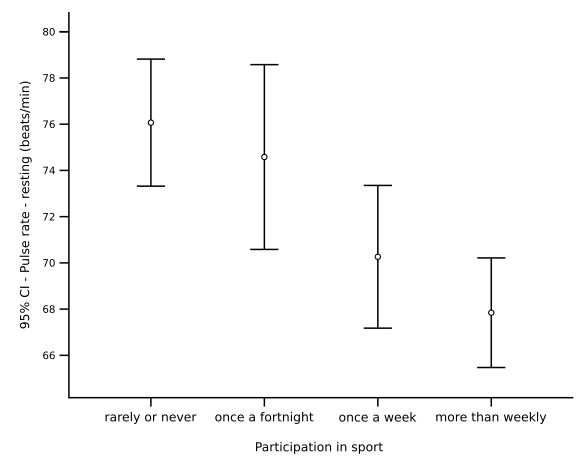
Bar markers with error bars depict means and their 95% confidence intervals. Such displays help judge overlap, relative precision, and whether observed differences are likely meaningful. Although the example shows pulse rate categories, the same presentation applies to physics measurements. Source

Data Processing Techniques

Processing converts raw readings into values that reveal relationships or validate hypotheses. Common techniques include:

• Averaging repeated measurements to reduce random errors.

• Calculating derived quantities such as gradients, ratios, or proportional constants.

• Converting non-linear data using mathematical transformations (e.g. taking logs to linearise an exponential relationship).

EQUATION
—-----------------------------------------------------------------
Mean (x̄) = (Σx) / n
x̄ = average value of data set
Σx = sum of all measurements
n = total number of measurements
—-----------------------------------------------------------------

Properly processed data improves the clarity of results and enhances their interpretability when compared to theoretical models.

Analysing Results

Identifying Patterns and Trends

Once data are processed, students must identify patterns, correlations, or proportional relationships. This analysis may involve:

• Recognising direct or inverse proportionality between variables.

• Detecting non-linear relationships and interpreting their physical meaning.

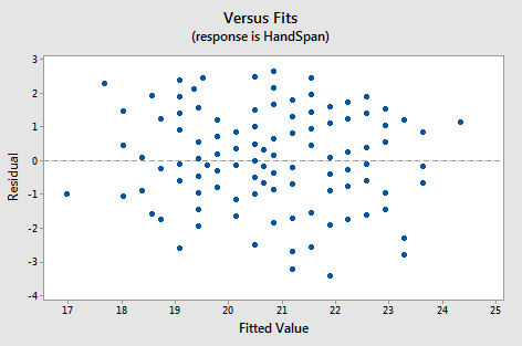
A residuals vs fits plot reveals whether residuals are randomly scattered about zero (good) or show patterns such as curvature or funneling. Such patterns suggest that the model form or error structure is inappropriate, guiding further processing (e.g., transformations). This diagnostic supports rigorous, evidence-based interpretation. Source

• Comparing experimental gradients or constants to theoretical expectations.

Trend analysis helps assess whether the experimental method effectively demonstrates the intended physical law.

Handling Quantitative and Qualitative Data

In Physics, results may be quantitative (numerical) or qualitative (descriptive).

• Quantitative analysis involves mathematical manipulation and statistical consideration.

• Qualitative interpretation focuses on observed behaviours such as phase changes, colour shifts, or directional changes of forces.

Both forms of data contribute to developing evidence-based conclusions, strengthening the reliability of findings.

Interpreting Quantitative Data

Calculating Gradients and Intercepts

Graphs are a vital analytical tool for identifying relationships. From a straight-line graph, one can calculate the gradient and y-intercept to extract physical quantities

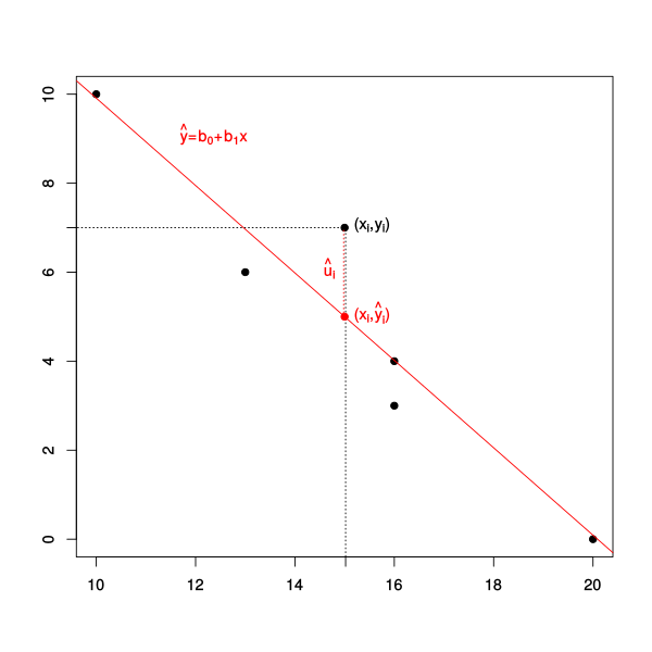
A scatter plot with a best-fit line illustrating how residuals represent the vertical difference between observed and predicted values. The labelled yiy_iyi​, y^i\hat y_iy^​i​, and residual highlight how quantitative interpretation links numerical outcomes to physical meaning. The diagram is minimal and directly aligned with A-level practical analysis. Source

EQUATION
—-----------------------------------------------------------------
Gradient (m) = Δy / Δx
m = rate of change between dependent and independent variables
Δy = change in dependent variable
Δx = change in independent variable
—-----------------------------------------------------------------

By comparing the measured gradient to a known theoretical value, students can test the accuracy of their experiment or determine unknown physical constants.

After calculating key values, interpretation should link numerical outcomes to physical meaning, explaining whether results support the hypothesis and why discrepancies might occur.

Propagating Uncertainties

To interpret results credibly, the propagation of uncertainty must be addressed. Combining multiple measurements increases total uncertainty, affecting confidence in conclusions.
When performing calculations:

• Add absolute uncertainties when quantities are added or subtracted.

• Add percentage uncertainties when quantities are multiplied or divided.

This ensures final results carry realistic margins of confidence and reflect measurement limitations.

Interpreting Qualitative Data

Observations and Descriptive Evidence

Qualitative data, though non-numerical, can be crucial in understanding physical phenomena. Descriptive notes about the behaviour of apparatus, appearance of materials, or consistency of trends help validate experimental logic.

When processing such data:

• Link each observation to theoretical principles.

• Identify whether visual changes support or contradict expectations.

• Consider whether environmental conditions influenced what was observed.

This interpretive reasoning deepens understanding and contextualises quantitative outcomes.

Drawing Evidence-Based Conclusions

From Data to Conclusion

A valid scientific conclusion is built upon processed evidence, not assumptions. Students must:

• Use analysed data to confirm or reject the hypothesis.

• Explain relationships between variables, including whether they align with theoretical predictions.

• Justify claims with numerical evidence, not anecdotal reasoning.

Each conclusion should directly address the experiment’s objective and acknowledge any sources of error or uncertainty that influence confidence in the outcome.

Validity, Reliability, and Accuracy

Interpreting results also involves judging their validity, reliability, and accuracy:

• Validity refers to whether the investigation measures what it intended to measure.

• Reliability describes the consistency of results when the experiment is repeated.

• Accuracy assesses closeness to the true or accepted value.

Evaluating these qualities demonstrates whether the experimental method supports credible scientific conclusions.

Connecting Data to Theory

Comparing Experimental and Theoretical Results

A key part of interpretation is comparing measured results with expected theoretical outcomes. Discrepancies may arise due to systematic errors, measurement limitations, or environmental effects.
When comparing:

• Calculate percentage difference between experimental and theoretical values.

• Assess whether differences lie within the expected uncertainty range.

• Offer reasoned explanations for deviations grounded in physics principles.

This comparison provides insight into the robustness of both the experiment and the theoretical model used.

EQUATION
—-----------------------------------------------------------------
Percentage Difference (%) = |Experimental – Theoretical| / Theoretical × 100
—-----------------------------------------------------------------

This simple calculation allows for direct evaluation of how closely results align with established physics, reinforcing the scientific integrity of interpretation.

Communicating Processed and Interpreted Results

Presenting Findings Clearly

Results should be communicated using concise, structured presentation:

• Include correctly labelled graphs and tables.

• Quote final answers with appropriate significant figures.

• Provide contextual interpretation explaining physical meaning and sources of uncertainty.

Effective communication ensures that data can be understood, verified, and replicated by others — a fundamental expectation of scientific practice.