
OCR Specification focus:
‘Estimate uncertainties and use graphs to analyse resistivity measurements.’
Uncertainty and data analysis are essential in resistivity experiments, helping physicists ensure results are accurate, reliable, and consistent with theoretical expectations. This topic focuses on identifying uncertainties, analysing graphs, and interpreting resistivity data with precision and clarity.
Understanding Uncertainty in Resistivity Measurements
In any experimental measurement, uncertainty represents the range within which the true value of a quantity is expected to lie. Every measured quantity — such as length, cross-sectional area, and resistance — contributes to the overall uncertainty in a calculated resistivity value. Recognising, estimating, and minimising these uncertainties are fundamental to achieving valid conclusions.
Sources of Uncertainty
Uncertainty in resistivity experiments arises from several key sources:
Instrument precision: Limited resolution of voltmeters, ammeters, micrometers, or rulers.
Human error: Parallax errors when reading scales, misalignment, or inconsistent readings.
Environmental factors: Temperature fluctuations can alter resistance, especially in metals.
Measurement technique: Poor electrical contacts, uneven wire thickness, or imperfect calibration.
Each of these must be identified and, where possible, quantified.
Absolute and Percentage Uncertainty
Absolute Uncertainty: The margin of error in a measurement, expressed in the same unit as the measured quantity.
For example, if a wire’s length is measured as 1.000 ± 0.005 m, the absolute uncertainty is ±0.005 m.
Percentage Uncertainty: The absolute uncertainty expressed as a percentage of the measured value.
Percentage uncertainty provides a convenient way to compare the relative reliability of measurements.
Calculating Uncertainty in Resistivity
The resistivity of a material is determined using the relationship between its resistance, length, and cross-sectional area.
EQUATION
—-----------------------------------------------------------------
Resistivity (ρ) = R A ÷ L
ρ = Resistivity (Ω m)
R = Resistance (Ω)
A = Cross-sectional area (m²)
L = Length (m)
—-----------------------------------------------------------------
When calculating the uncertainty in resistivity, students must combine the uncertainties from all measured quantities. The rule for combining percentage uncertainties applies when quantities are multiplied or divided:
Total percentage uncertainty in ρ = % uncertainty in R + % uncertainty in A + % uncertainty in L
This process highlights which measurement contributes most to the overall uncertainty, allowing focus on improving experimental accuracy.
Reducing Uncertainty
To minimise uncertainty:
Take multiple readings and calculate a mean value.
Use high-precision instruments (e.g., digital micrometers for diameter).
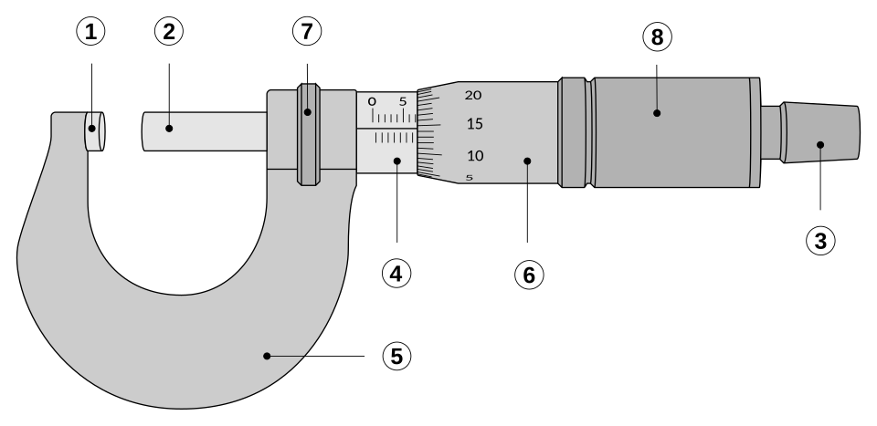
A labelled micrometer caliper showing a metric reading and indicated reading uncertainty (±0.005 mm). This diagram models good practice for measuring wire diameter repeatedly to reduce percentage uncertainty in area. Extra detail beyond the syllabus is limited to naming individual parts of the micrometer, which is acceptable background. Source.
Maintain constant temperature to avoid resistance fluctuations.
Ensure good electrical contact to reduce connection resistance.
Keep wires straight and untwisted to maintain uniform cross-section.
Consistent measurement practices significantly improve the reliability of resistivity results.
Analysing Data Using Graphs
Graphical analysis provides a powerful way to interpret data and identify patterns in resistivity measurements. It helps determine the linearity between variables and detect systematic errors.
Plotting Resistance Data
In a typical resistivity investigation:
A wire’s resistance R is measured for different lengths L.
A graph of R against L is plotted.
The gradient of the line is then used to calculate resistivity.
EQUATION
—-----------------------------------------------------------------
Gradient (m) = ΔR ÷ ΔL
R = Resistance (Ω)
L = Length (m)
—-----------------------------------------------------------------
From the gradient, resistivity can be found using:
EQUATION
—-----------------------------------------------------------------
ρ = (Gradient × A)
ρ = Resistivity (Ω m)
A = Cross-sectional area (m²)
—-----------------------------------------------------------------
The graph should pass through the origin if resistance is directly proportional to length, confirming the expected linear relationship for a uniform conductor.
Identifying and Representing Uncertainties on Graphs
When plotting data, error bars are used to represent the uncertainty in each measurement:
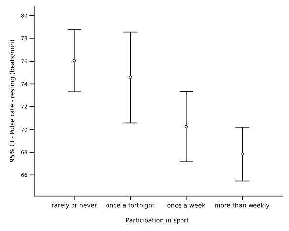
Vertical error bars indicate the uncertainty range for each plotted value. This reinforces how confidence intervals or other uncertainty measures are shown on graphs used to analyse resistivity data. The underlying data (pulse rate vs exercise level) is not part of the physics syllabus but the error-bar convention is identical and transferable to R–L plots. Source.
Vertical error bars show uncertainty in resistance (R).
Horizontal error bars show uncertainty in length (L).
Error bars visually indicate the confidence range for each data point. A line of best fit should pass as close as possible to all points, with approximately equal scatter above and below it.
If data points do not align well with a straight line, this may suggest:
Measurement errors or incorrect assumptions.
Temperature variations affecting resistance.
Non-uniform wire thickness or poor contacts.
Using Lines of Best and Worst Fit
To estimate uncertainty in the gradient:
Draw a best-fit line through the data.
Draw maximum and minimum gradients (worst-fit lines) that still pass within all error bars.
Calculate the percentage uncertainty in the gradient as:
(Δm÷m)×100(Δm ÷ m) × 100%(Δm÷m)×100
where Δm is the difference between the maximum and minimum gradient divided by two.
This provides a clear estimate of how measurement scatter affects the calculated resistivity.
Evaluating Experimental Data
Critical analysis of resistivity data ensures scientific integrity. Students should:
Compare experimental results with accepted values to assess accuracy.
Identify and justify any anomalous results.
Consider whether systematic errors (such as calibration drift or heating effects) influenced outcomes.
Quantify overall uncertainty in the final resistivity value using propagated errors.
By evaluating both random and systematic uncertainties, physicists can report results that are both quantitatively justified and scientifically valid.
Reporting Results
Results should be presented as:
ρ = (value ± uncertainty) Ω m
This communicates both the measured resistivity and the range within which the true value is likely to lie, satisfying the OCR requirement to estimate uncertainties and use graphs to analyse resistivity measurements.
Practice Questions
Question 1 (2 marks)
A student measures the length of a wire as 1.200 ± 0.005 m.
(a) Calculate the percentage uncertainty in the length.
(b) State one way the student could reduce this uncertainty.
Mark Scheme
(a) Percentage uncertainty = (0.005 ÷ 1.200) × 100 = 0.42% (1 mark)
(b) Any one of the following:
Use a ruler or measuring device with finer scale divisions.
Take multiple measurements and calculate a mean.
Ensure the wire is straight and taut before measuring.
(1 mark for any valid method)
Question 2 (5 marks)
In an experiment to determine the resistivity of a metal wire, a student measures the resistance of wires of different lengths. The graph of resistance (R) against length (L) is a straight line through the origin with a gradient of 0.045 Ω m⁻¹. The cross-sectional area of the wire is (1.0 ± 0.1) × 10⁻⁶ m².
(a) Calculate the resistivity of the wire.
(b) Estimate the percentage uncertainty in the resistivity, stating the main source of uncertainty.
(c) Suggest one improvement to reduce the overall uncertainty in the experiment.
Mark Scheme
(a) Use ρ = gradient × A
ρ = 0.045 × 1.0 × 10⁻⁶ = 4.5 × 10⁻⁸ Ω m (1 mark)
(b) Percentage uncertainty in resistivity = % uncertainty in gradient + % uncertainty in A
Assume uncertainty in gradient negligible, so main contribution is from A (10%)
Percentage uncertainty ≈ 10% (2 marks)
Main source of uncertainty: measurement of wire diameter (used to find A) (1 mark)
(c) Valid improvement such as:
Use a micrometer to measure diameter at several points and take a mean.
Use thicker wire to reduce relative uncertainty in diameter.
Keep wire at constant temperature to avoid resistance drift.
(1 mark for any valid suggestion)
FAQ
Random uncertainties cause unpredictable fluctuations in readings, such as small variations when measuring resistance or length. They can be reduced by taking multiple readings and calculating a mean.
Systematic uncertainties consistently shift all readings in one direction, such as an incorrectly calibrated voltmeter or a micrometer with a zero error. These cannot be reduced by repetition and must be identified and corrected through calibration or comparison with a standard.
Temperature changes can significantly alter resistance, particularly for metals where resistivity increases with temperature. Even a small rise from heating by current flow introduces additional uncertainty.
To minimise this:
Use low currents to reduce heating.
Allow time between readings for cooling.
Record ambient temperature and note its effect on results.
Maintaining stable conditions improves both accuracy and repeatability.
Thin wires have very small diameters, often close to the micrometer’s resolution limit. Any small error in reading the scale or imperfect contact pressure causes a large percentage uncertainty.
In addition, slight variations in wire thickness along its length increase uncertainty in cross-sectional area calculations.
To counter this:
Measure diameter at several points and take the mean.
Rotate the wire during measurement to avoid bias from irregularities.
Systematic errors often appear as consistent deviations from expected linear trends. For example, if the R–L graph does not pass through the origin, this indicates a constant offset, possibly due to contact resistance or poor connections.
To investigate:
Check the intercept of the graph.
Ensure all apparatus is zeroed correctly.
Re-test with new connections or leads.
Recognising such trends on graphs helps correct or account for systematic errors.
Resistivity results should always include both the calculated value and its uncertainty. Present them in the form:
ρ = (value ± absolute uncertainty) Ω m
For example, ρ = (1.68 ± 0.08) × 10⁻⁸ Ω m.
Alternatively, a percentage uncertainty may be stated in brackets, e.g., ρ = (1.68 × 10⁻⁸ Ω m) ± 5%.
This format clearly communicates the precision and reliability of the measured resistivity.
