
OCR Specification focus:
‘Use an oscilloscope to determine frequency of signals and waves.’
Oscilloscopes are essential instruments in physics and engineering that allow the visualisation and measurement of time-varying signals. In A-Level Physics, they are used to determine the frequency, amplitude, and waveform of electrical signals and to relate these to the properties of progressive waves.
Understanding the Oscilloscope
An oscilloscope is a device that displays how voltage varies with time. The resulting trace (or waveform) appears on a screen where the horizontal axis represents time and the vertical axis represents potential difference (voltage). By examining this trace, physicists can extract key information about the behaviour of waves, including their frequency and period.
Basic Components
An oscilloscope typically includes:
Cathode ray tube (CRT) or digital display to show the waveform.
Time base control to adjust the scale of the horizontal axis.
Y-gain control to set the vertical scale (voltage per division).
Trigger control to stabilise the waveform on the screen.
Input channel(s) for connecting the signal source, such as a signal generator or microphone.
These controls must be carefully adjusted to obtain a stable and measurable waveform.
Display Axes and Calibration
The oscilloscope screen is divided into a grid of divisions—horizontal and vertical boxes. Each division corresponds to a specific time or voltage scale, set by the user.
Calibration Controls
The time base determines how much time each horizontal division represents (e.g. 1 ms per division).
The Y-gain sets how much voltage each vertical division represents (e.g. 2 V per division).
By counting divisions between specific waveform points, measurements can be converted into meaningful quantities such as period and amplitude.
Measuring the Period and Frequency
The period (T) of a wave is the time taken for one complete cycle of the waveform. On the oscilloscope, this is the distance between two successive identical points on the trace (for example, two consecutive peaks).
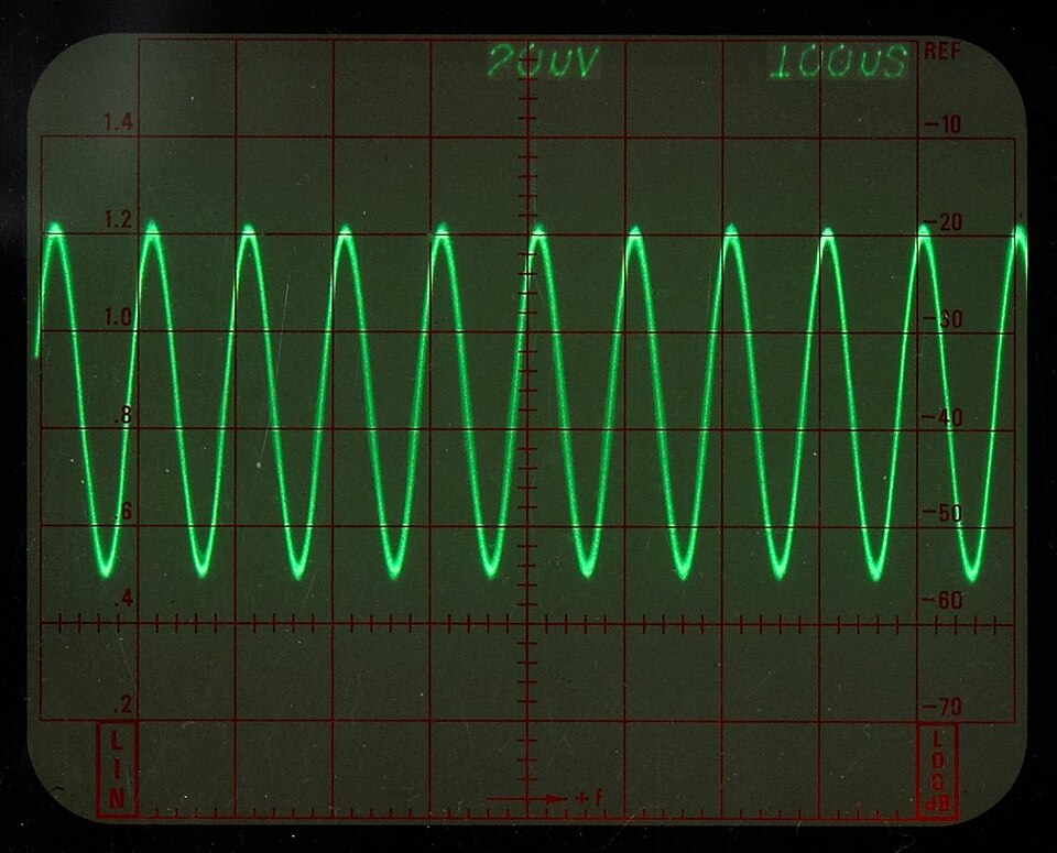
Sine-wave trace on a Tektronix analogue oscilloscope with calibrated graticule. The horizontal scale (seconds per division) lets you read off the period across one cycle; the vertical scale (volts per division) gives the amplitude. The small on-screen readouts across the top show the active time-base and vertical sensitivity settings used. Source.
EQUATION
—-----------------------------------------------------------------
Time–Frequency Relationship (f = 1/T)
f = 1 / T
f = Frequency of the signal, measured in hertz (Hz)
T = Period of the waveform, measured in seconds (s)
—-----------------------------------------------------------------
To determine frequency using the oscilloscope:
Measure the horizontal length of one complete cycle on the screen in divisions.
Multiply this number by the time base setting to find the period (T).
Use the equation above to calculate frequency (f).
For instance, if one cycle spans 5 divisions and the time base is 0.2 ms/division, then T = 5 × 0.2 ms = 1.0 ms, and f = 1 / 1.0 × 10⁻³ = 1.0 kHz.
Displaying and Measuring Amplitude
Amplitude refers to the maximum displacement of the signal from its mean (zero) line, corresponding to the peak voltage.
Amplitude: The maximum value of displacement or voltage from the equilibrium (zero) position of a wave.
The vertical distance between the waveform’s peak and trough gives the peak-to-peak voltage, which equals twice the amplitude. Measuring this distance in divisions and multiplying by the Y-gain setting provides the actual amplitude in volts.
Measuring Two Signals: Frequency Comparison
Oscilloscopes can display two signals simultaneously using dual-trace mode. This allows for direct comparison between signals, such as an input and output from a system.
If both signals have the same frequency, their cycles align consistently.
A difference in phase or frequency is visible as a gradual shift in alignment.
Phase Difference: The amount by which one wave is shifted relative to another, often expressed as an angle (degrees or radians).
When measuring the frequency of an unknown signal, it can be compared with a known reference from a signal generator. The oscilloscope helps to adjust and match frequencies until their traces synchronise.
Lissajous Figures and Frequency Determination
When two signals are applied to the X and Y inputs of an oscilloscope, rather than time and voltage respectively, the resulting pattern is a Lissajous figure.
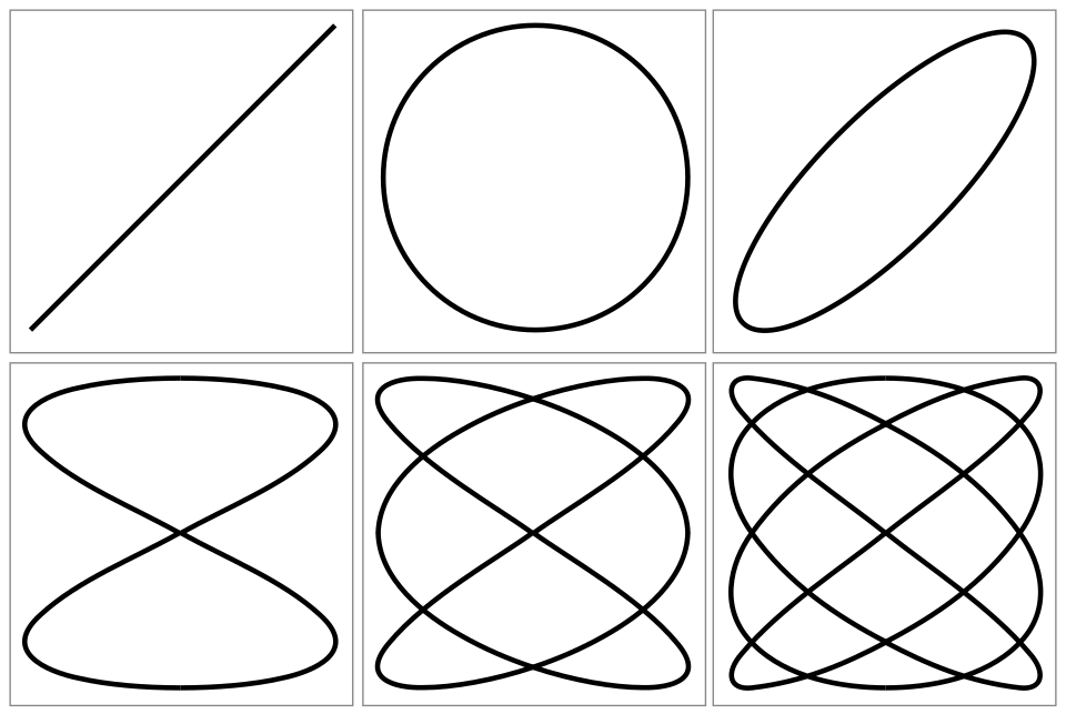
A set of canonical Lissajous curves produced by sinusoidal signals applied to perpendicular axes. Stationary, closed patterns indicate simple frequency ratios (e.g., 1:1, 2:1, 3:2) and allow frequency comparison when one source is known. This figure includes several phase/ratio cases; some patterns exceed the minimal example needed but remain instructive. Source.
The shape of this figure depends on the frequency ratio and phase relationship between the two signals.
A stationary, repeating pattern indicates a simple frequency ratio, such as 1:1 or 2:1.
The ratio of the number of loops along each axis provides the frequency ratio of the two signals.
This technique is particularly useful when one frequency is unknown but the other is accurately calibrated.
Practical Use: Measuring Audio and Wave Signals
Oscilloscopes are invaluable for examining sound waves, electromagnetic waves, and electrical signals indirectly converted into electrical form using transducers such as microphones.
For instance:
A microphone converts sound waves into electrical oscillations displayed as voltage-time traces.
The frequency of the sound can then be determined by measuring the trace period and applying f = 1/T.
To ensure accuracy:
Set the time base so that several complete cycles fit neatly across the screen.
Use trigger controls to stabilise the display.
Average multiple readings to reduce human error in counting divisions.
Limitations and Sources of Error
Although highly effective, oscilloscope readings can be influenced by several factors:
Calibration drift in time base or Y-gain controls leading to inaccurate scales.
Parallax error when reading screen divisions at an angle.
Signal noise distorting the waveform, making period measurement difficult.
Aliasing if the sampling rate in digital oscilloscopes is too low for the signal frequency.
To minimise these, users should regularly calibrate instruments, ensure signal stability, and make multiple measurements for consistency.
Key Takeaways for OCR A-Level Physics
Understanding how to use an oscilloscope to determine frequency links directly to experimental skills within the Waves topic. It combines theoretical knowledge of wave equations with practical instrumentation techniques. Mastery of this subsubtopic enables accurate measurement of frequency, amplitude, and phase, underpinning experimental work involving sound, microwaves, and other progressive waves.
Practice Questions
Question 1 (2 marks)
An oscilloscope is used to display a signal from a signal generator. The time base is set to 0.5 ms per division, and one complete cycle of the waveform spans 4 divisions horizontally.
Calculate the frequency of the signal.
Mark Scheme:
Correct calculation of period: T = 4 × 0.5 ms = 2.0 ms (1 mark)
Correct calculation of frequency: f = 1 / 2.0 × 10⁻³ = 500 Hz (1 mark)
Question 2 (5 marks)
A student uses an oscilloscope to investigate an alternating current (a.c.) signal from a microphone connected to the Y-input. The oscilloscope is set up so that the waveform fills most of the screen vertically and several cycles are visible horizontally.
(a) Explain how the student should adjust the oscilloscope controls to obtain a clear and stable waveform. (3 marks)
(b) Describe how the student can use the oscilloscope trace to determine the frequency of the sound detected by the microphone. (2 marks)
Mark Scheme:
(a) (3 marks total)
Adjust the time base (seconds per division) so that one or more complete cycles are visible and measurable. (1 mark)
Adjust the Y-gain (volts per division) so the waveform fits vertically on the screen without clipping. (1 mark)
Use the trigger control to stabilise the trace and prevent it from drifting across the screen. (1 mark)
(b) (2 marks total)
Measure the horizontal length (number of divisions) of one complete cycle on the trace. (1 mark)
Multiply by the time base setting to find the period (T), then use f = 1/T to calculate the frequency. (1 mark)
FAQ
Analogue oscilloscopes display the waveform in real time using a cathode ray tube, so frequency is measured directly from the continuous trace.
Digital oscilloscopes, on the other hand, sample the signal at discrete intervals and reconstruct the waveform electronically. This allows for automatic frequency measurement, data storage, and signal analysis. However, if the sampling rate is too low, aliasing may occur, where the displayed waveform has an incorrect apparent frequency.
To prevent this, the sampling frequency should be at least twice the signal frequency (the Nyquist criterion).
Without triggering, the waveform may drift horizontally across the screen, making accurate period measurement impossible.
The trigger control synchronises the start of the sweep with a particular point on the waveform, such as when the signal crosses zero volts in a rising direction.
By maintaining a stable starting point, the waveform appears stationary, allowing you to count divisions and determine the period (and therefore the frequency) accurately.
Different trigger modes—auto, normal, or single—control how the oscilloscope responds when no valid trigger signal is detected.
To reduce human and instrument error:
Adjust the time base so that several full cycles fill the screen.
Use fine time-base controls to optimise trace length.
Take multiple readings of period and average them.
Ensure instrument calibration is up to date.
Minimise parallax error by viewing the trace straight on.
Digital oscilloscopes may also include cursors or on-screen readouts that display the time interval directly, improving precision over manual counting.
If the time base is too fast (too few seconds per division), only part of a cycle will be visible, preventing period measurement.
If it is too slow (too many seconds per division), several cycles will overlap or compress, making the trace difficult to interpret.
An appropriately chosen time-base setting ensures that one to three full cycles fit neatly across the screen, giving a clear, measurable waveform suitable for accurate frequency determination.
Yes. The upper measurable frequency depends on the oscilloscope’s bandwidth—the highest frequency the device can display accurately.
Typical laboratory oscilloscopes for A-Level use have bandwidths in the range of 20–50 MHz, allowing them to measure much higher frequencies than human hearing (20 kHz).
However, at frequencies approaching the oscilloscope’s limit, signals may appear distorted or attenuated, leading to errors in frequency measurement. For such cases, specialised high-bandwidth or sampling oscilloscopes are used.
