
OCR Specification focus:
‘Relate displacement, velocity and acceleration graphs to interpret simple harmonic motion.’
Simple harmonic motion (SHM) can be understood visually through graphs that show how displacement, velocity, and acceleration vary with time or displacement. These graphical relationships illustrate how these quantities are interrelated in both phase and magnitude. Understanding these graphs enables students to connect equations of motion to observable oscillatory behaviour.
Displacement–Time Graphs
A displacement–time graph shows how an oscillating object’s position varies over time. The displacement, represented by x, oscillates about the equilibrium position, alternating between maximum positive and negative values.
Displacement (x): The distance and direction of an oscillating object from its equilibrium position at any instant.
For a simple harmonic oscillator, the displacement follows a sinusoidal pattern. The curve can be represented mathematically as either x = A sin(ωt) or x = A cos(ωt + φ), depending on the starting condition of motion. The shape of the graph resembles a smooth wave, symmetric about the equilibrium line.
Key features of the displacement–time graph:
The amplitude (A) is the maximum displacement from the equilibrium position.
The period (T) is the time taken for one complete oscillation.
The frequency (f) is the number of oscillations per second.
EQUATION
—-----------------------------------------------------------------
Angular frequency (ω) = 2πf = 2π / T
ω = Angular frequency (rad s⁻¹)
f = Frequency (Hz)
T = Period (s)
—-----------------------------------------------------------------
At maximum displacement, the velocity is zero, and at the equilibrium position, displacement is zero but velocity is maximum.
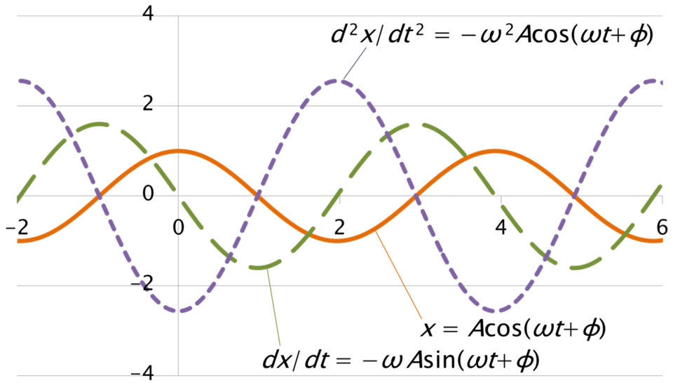
Displacement x(t)x(t)x(t), velocity v(t)v(t)v(t), and acceleration a(t)a(t)a(t) for simple harmonic motion plotted against time. The curves share the same period but differ in phase: velocity leads displacement by 90∘90^\circ90∘, and acceleration is 180∘180^\circ180∘ out of phase with displacement. Axes and labels are minimal and clear to emphasise the phase shifts. Source.
These relationships become clearer when comparing the velocity–time and acceleration–time graphs.
Velocity–Time Graphs
The velocity–time graph for SHM is also sinusoidal but shifted in phase relative to the displacement–time graph. Velocity reaches its maximum when the displacement crosses zero and becomes zero at the extremes of motion.
Velocity (v): The rate of change of displacement with respect to time; it indicates both the speed and direction of motion.
In SHM:
Velocity leads displacement by 90° (π/2 radians) in phase.
The velocity graph has the same period and frequency as the displacement graph.
The velocity is positive when the object moves towards the equilibrium position from the negative side and negative when moving away.
EQUATION
—-----------------------------------------------------------------
Velocity in SHM (v) = ±ω√(A² − x²)
v = Velocity (m s⁻¹)
ω = Angular frequency (rad s⁻¹)
A = Amplitude (m)
x = Displacement (m)
—-----------------------------------------------------------------
At equilibrium (x = 0), the velocity is at its maximum value vₘₐₓ = ωA. This relationship helps explain how kinetic energy varies during the motion.
Acceleration–Time Graphs
The acceleration–time graph mirrors the displacement–time graph but is inverted, showing that acceleration and displacement are always in opposite directions. This inverse relationship is a defining property of SHM.
Acceleration (a): The rate of change of velocity with respect to time; in SHM, it acts towards the equilibrium position and is proportional to displacement.
The mathematical form of acceleration in SHM is given by:
EQUATION
—-----------------------------------------------------------------
Defining Equation of SHM: a = −ω²x
a = Acceleration (m s⁻²)
ω = Angular frequency (rad s⁻¹)
x = Displacement (m)
—-----------------------------------------------------------------
This equation shows that acceleration is directed opposite to displacement and proportional to it, reinforcing the restoring nature of SHM. When the object is furthest from equilibrium (x = ±A), acceleration is maximum and directed towards the centre.
Phase Relationships Between Graphs
Understanding phase difference is essential to interpreting SHM graphs accurately.
Displacement and acceleration are 180° (π radians) out of phase. When displacement is at a maximum, acceleration is maximum but in the opposite direction.
Velocity is 90° out of phase with both displacement and acceleration, lying midway between their extrema.
These phase differences can be visualised by comparing the three time-based graphs:
When x = +A, v = 0, a = −ω²A.
When x = 0, v = +ωA, a = 0.
When x = −A, v = 0, a = +ω²A.
Such relationships are key to understanding how energy interchanges between kinetic and potential forms in later sections.
Displacement–Velocity and Displacement–Acceleration Graphs
Besides time graphs, it is useful to plot velocity versus displacement and acceleration versus displacement.
A velocity–displacement (v–x) graph forms an ellipse, as v² = ω²(A² − x²). This representation shows that velocity decreases as displacement increases.
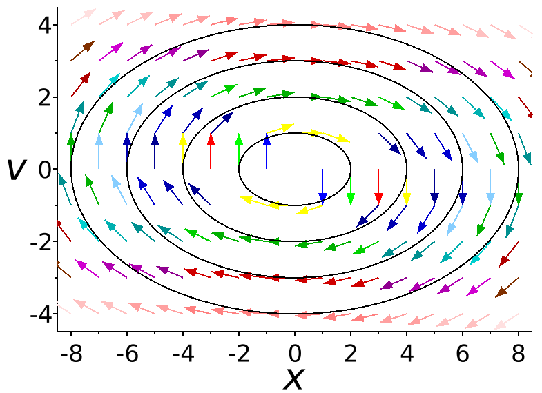
Phase plane for a simple harmonic oscillator with vvv on the vertical axis and xxx on the horizontal axis. Closed elliptical orbits correspond to constant-amplitude SHM; arrows indicate the direction of motion as time progresses. This static vector-field view reinforces that speed is greatest near x=0x=0x=0 and zero at ∣x∣=A|x|=A∣x∣=A. Source.
An acceleration–displacement (a–x) graph is a straight line with a negative gradient, demonstrating direct proportionality between acceleration and displacement but in opposite directions.
The linear a–x graph provides an experimental confirmation of SHM since its slope equals −ω². This can be used to determine the angular frequency of the oscillation in practical investigations.
Interpreting Graphical Data in Experiments
In laboratory work, oscillatory data can be collected using motion sensors or light gates. Plotting displacement, velocity, and acceleration graphs allows identification of SHM behaviour:
The sinusoidal displacement curve confirms periodic motion.
The 90° phase shift between displacement and velocity confirms harmonic oscillation.
The linear a–x relationship validates the proportional restoring force.
Students should note:
Graphs of displacement vs time reveal period and amplitude.
Velocity vs time graphs indicate phase shifts and maximum speed.
Acceleration vs time graphs demonstrate restoring behaviour and allow estimation of angular frequency.
Through careful interpretation of these graphs, the defining characteristics of SHM — periodicity, sinusoidal form, and proportional restoring acceleration — become clearly evident. These relationships underpin much of the analysis used in oscillatory physics, from pendulums and springs to atomic and electrical systems.
Practice Questions
Question 1 (2 marks)
Describe the phase relationship between displacement and velocity for a particle undergoing simple harmonic motion (SHM).
Mark scheme:
1 mark: States that velocity leads displacement by 90° (or π/2 radians).
1 mark: States that velocity is zero when displacement is maximum and maximum when displacement is zero.
Question 2 (5 marks)
A student observes the motion of a simple harmonic oscillator and records the variation of displacement, velocity, and acceleration with time.
Explain how the shapes and relative phases of the three quantities on the time axis confirm that the motion is simple harmonic.
Mark scheme:
1 mark: Identifies that all three quantities vary sinusoidally with time.
1 mark: States that velocity leads displacement by 90° (or π/2 radians).
1 mark: States that acceleration is in antiphase (180° out of phase) with displacement.
1 mark: Mentions that the amplitude of acceleration is proportional to displacement (a = –ω²x).
1 mark: Concludes that the restoring acceleration always acts towards the equilibrium position, consistent with SHM.
FAQ
The shape of the displacement–time graph depends on the initial conditions of the oscillation. If the object starts from its maximum displacement, the graph follows a cosine shape (x = A cos ωt). If it starts from the equilibrium position, it follows a sine shape (x = A sin ωt).
In both cases, the graph is sinusoidal, symmetrical about the equilibrium line, and repeats after one complete period.
Acceleration is produced by a restoring force that acts towards the equilibrium position. Since displacement measures how far the object is from equilibrium, the restoring acceleration must always act to reduce this displacement.
This is expressed mathematically as a = −ω²x, where the negative sign indicates that acceleration is directed opposite to displacement.
Plotting acceleration (a) against displacement (x) gives a straight line through the origin with a negative gradient if the motion is simple harmonic.
This linear relationship demonstrates that acceleration is directly proportional to and in the opposite direction of displacement. The slope of the line provides −ω², allowing the angular frequency to be calculated experimentally.
Phase differences show how one quantity reaches its maximum or zero value relative to another.
Displacement and velocity are 90° out of phase.
Displacement and acceleration are 180° out of phase.
Velocity reaches its maximum when displacement is zero, helping identify direction and timing of motion from graphs.
Recognising these phase shifts is essential for interpreting experimental and theoretical SHM data correctly.
The elliptical shape arises because the relationship between velocity and displacement follows v² = ω²(A² − x²).
As displacement increases towards ±A, velocity decreases to zero, forming the curved boundary of an ellipse.
A circular plot would only appear if both axes were scaled differently to equalise units, but in SHM, differing dimensions (m vs m s⁻¹) produce a natural ellipse.
