
OCR Specification focus:
‘Describe damping’s effect on amplitude; observe forced and damped oscillations experimentally.’
Damping in oscillatory systems reduces energy and amplitude over time through resistive forces. Understanding damping is essential for analysing real-world oscillations and predicting system behaviour.
Understanding Damping in Oscillations
All real oscillating systems lose energy to their surroundings. Damping refers to any process that dissipates energy from an oscillating system, typically through frictional, viscous, or resistive forces. These forces act in the opposite direction to motion and gradually reduce the amplitude of oscillation.
Damping: The effect of a resistive force that causes the energy of an oscillating system to decrease over time, reducing its amplitude.
Damping transforms mechanical energy into heat or sound energy, meaning the oscillator’s total mechanical energy continually decreases. The rate of this decay depends on the magnitude and type of damping force present.
Types of Damping
There are three main types of damping that students must recognise: light damping, critical damping, and heavy (over) damping.
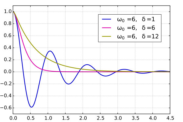
A displacement–time plot comparing underdamped (oscillatory decay), critically damped (fastest non-oscillatory return), and overdamped (slow non-oscillatory return) responses. The curves show how increasing damping removes overshoot and lowers the amplitude more rapidly. Labels and axes are uncluttered for quick comparison. Source.
Each has distinct effects on amplitude and motion.
Light Damping
In lightly damped systems, resistive forces are small. The amplitude decreases gradually with time, and oscillations continue for many cycles before stopping.
The system still oscillates about the equilibrium position.
The period remains almost unchanged compared to undamped motion.
Energy loss per cycle is small but cumulative.
This type of damping is typical of air resistance acting on a pendulum or mechanical spring.
Mathematically, amplitude decreases exponentially over time.
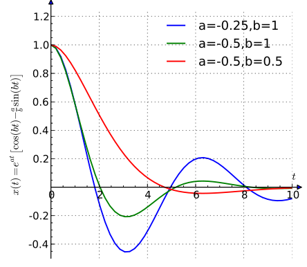
Displacement–time graph of a damped oscillator with the exponential envelope highlighted. The envelope visualises how amplitude falls by a constant fraction per equal time interval under viscous damping. This directly supports exponential decay modelling used in lab analysis. Source.
EQUATION
—-----------------------------------------------------------------
Amplitude decay (A) = A₀ e^(−kt)
A₀ = Initial amplitude (m)
k = Damping coefficient (s⁻¹)
t = Time (s)
—-----------------------------------------------------------------
This relationship shows how amplitude diminishes with time, while frequency and period remain nearly constant for light damping.
Critical Damping
Critical damping occurs when the resistive force is exactly large enough to prevent oscillations altogether, but allows the system to return to equilibrium in the shortest possible time.
The system does not overshoot its equilibrium position.
It returns to rest quickly, without oscillating.
Common in car suspension systems and measuring instruments like galvanometers.
This condition represents the boundary between oscillatory and non-oscillatory motion.
Heavy (Over) Damping
When the resistive forces are too large, heavy damping occurs.
The system returns to equilibrium without oscillating, but much more slowly than in the critically damped case.
Motion is sluggish and overdamped systems respond poorly to rapid changes.
Found in door closers or shock absorbers designed for slow, steady return.
Thus, increasing damping beyond the critical value no longer improves response time but delays motion.
Damping and Amplitude Reduction
The defining feature of damping is its effect on amplitude. As energy is lost, the maximum displacement from equilibrium reduces over time. Because kinetic and potential energy are proportional to amplitude squared, even small damping forces can significantly lower total energy.
In free oscillations (no external driving force), amplitude decays continuously until motion stops. The system’s natural frequency also decreases slightly if damping is significant, though for light damping the effect on frequency is negligible.
Amplitude-time graphs for damped motion show progressively smaller peaks.
Each successive peak is a fixed fraction of the previous one, consistent with exponential decay.
Energy-time graphs display a faster reduction since energy ∝ amplitude².
Damping in Forced Oscillations
When an external periodic force acts on a system, it produces forced oscillations. The amplitude of these oscillations depends strongly on the driving frequency and the extent of damping.
With no damping, the amplitude would theoretically become infinite at resonance.
With light damping, the amplitude still peaks near the natural frequency, but remains finite.
With greater damping, the resonance peak becomes lower and broader, meaning the system responds less sharply to frequency changes.
Therefore, damping prevents destructive resonance and ensures stability in practical systems.
Experimental Observation of Damping
Students must be able to observe and describe damping experimentally.
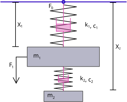
Schematic of a mass–spring–damper system, the standard model for studying damping in the lab. The dashpot represents the resistive force that dissipates energy and reduces amplitude over time. Diagram is intentionally minimal to emphasise the key elements only. Source.
Typical laboratory investigations use mechanical or electrical oscillators and measure amplitude decay over time.
Experimental Methods
Mass–spring system: Track displacement using a motion sensor or ruler as oscillations decay.
Torsional pendulum: Record angular displacement over successive oscillations.
Oscilloscope observation: In electrical oscillators, observe voltage amplitude decreasing with time.
Key Experimental Features
Measure amplitude or peak height at successive cycles.
Plot ln(A) against time (t) to verify exponential decay; the gradient gives the damping coefficient (k).
Repeat with different damping materials or fluids to compare rates of decay.
These experiments reinforce the quantitative relationship between damping and amplitude reduction.
Practical Importance of Damping
Damping is essential in engineering and design because it controls vibrations and ensures system stability. Understanding its effects allows engineers to balance responsiveness with safety and durability.
Examples include:
Vehicle suspension systems using critical damping for smooth rides.
Building design employing dampers to reduce earthquake-induced oscillations.
Instrument needles damped to prevent overshoot and allow rapid stable readings.
Excessive or insufficient damping can cause performance issues: underdamped systems oscillate too long, while overdamped systems respond too slowly. Hence, the appropriate level of damping must be selected according to the application.
Quantitative and Qualitative Analysis
From a quantitative perspective, damping affects measurable quantities such as amplitude, energy, and rate of decay. Qualitatively, it changes the appearance of displacement–time graphs:
Light damping: smoothly decaying sinusoidal pattern.
Critical damping: curve returning swiftly to equilibrium without oscillation.
Heavy damping: gradual non-oscillatory return to equilibrium.
In all cases, damping reduces amplitude and dissipates energy, aligning precisely with the OCR specification requirement to “describe damping’s effect on amplitude” and “observe forced and damped oscillations experimentally.”
Practice Questions
Question 1 (2 marks)
Explain how damping affects the amplitude of oscillations in a simple harmonic oscillator.
Mark Scheme:
1 mark for stating that damping causes the amplitude of oscillations to decrease with time.
1 mark for identifying that this occurs because energy is dissipated (e.g. by frictional or resistive forces).
Question 2 (5 marks)
A student investigates the effect of damping on a mass–spring system. The amplitude of oscillation is measured over time, and it is found to decrease exponentially.
(a) State one reason why the amplitude decreases exponentially rather than linearly. (1 mark)
(b) Explain how increasing the damping coefficient affects:
(i) the amplitude of successive oscillations,
(ii) the time taken to return to equilibrium,
(iii) the frequency of oscillation. (4 marks total)
Mark Scheme:
(a)
1 mark: The resistive force (or energy loss) is proportional to velocity, leading to exponential decay of amplitude.
(b)
(i)
1 mark: Increasing the damping coefficient increases the rate of energy loss, so amplitude decreases more rapidly between successive oscillations.
(ii)
1 mark: For heavy damping, the system returns to equilibrium without oscillating, and the return time increases as damping becomes greater.
(iii)
1 mark: The frequency decreases slightly with increased damping, but for light damping the change is negligible.
1 additional mark for a clear, coherent explanation linking damping to energy dissipation and motion behaviour.
FAQ
The rate of damping depends on how efficiently energy is transferred from the oscillating system to its surroundings. Key factors include:
The nature of the medium — air, water, or oil all provide different levels of resistive force.
The surface area and shape of the oscillating object, affecting drag.
The viscosity of the medium for fluid damping.
The presence of internal friction within materials or joints.
A larger damping coefficient corresponds to greater energy loss per cycle and faster amplitude reduction.
In heavy damping, the resistive force is so large that it opposes motion almost immediately after displacement. This high resistance prevents the system from overshooting its equilibrium position.
Instead of oscillating back and forth, the object moves slowly and directly toward equilibrium. Although it eventually settles, the motion is sluggish and non-periodic because the restoring force is continually opposed by significant energy loss through damping.
Reducing damping helps obtain more accurate measurements of natural frequency and period. To minimise damping:
Use low-friction pivots or bearings.
Conduct experiments in air rather than water to lower viscous resistance.
Ensure materials are rigid and well-lubricated to reduce internal friction.
Avoid attachments that absorb or dissipate energy, such as loose clamps.
Controlling environmental factors like air currents and vibration also helps limit unwanted damping effects.
The damping coefficient, often denoted by k, quantifies the rate of amplitude decay. To determine it experimentally:
Measure successive peak amplitudes of a free oscillation.
Plot ln(A) against time (t) — the resulting line should be straight.
The gradient equals –k, allowing direct calculation.
Alternatively, electronic or sensor-based systems can record decay curves for precise data analysis in both mechanical and electrical oscillators.
Damping prevents resonance from producing excessive amplitudes by dissipating energy from the system as heat or sound.
In undamped or lightly damped systems, the energy from a driving force accumulates rapidly at the natural frequency, causing very large oscillations.
With damping present:
The resonance peak becomes lower and broader.
The system responds over a wider range of frequencies with smaller amplitudes.
This controlled response is crucial for safety in bridges, vehicles, and machinery, where unchecked resonance could cause structural failure.
