
OCR Specification focus:
‘Interpret amplitude versus driving frequency graphs for damped, forced oscillators.’
Understanding amplitude–frequency response is essential for analysing how oscillators react to varying driving frequencies, particularly when damping is present, revealing characteristic changes in amplitude and resonance behaviour.
The Nature of Amplitude–Frequency Response
The amplitude–frequency response describes how the steady-state amplitude of a forced oscillator varies with the driving frequency of an external periodic force. When damping is present, the shape and height of the response curve change significantly, and this provides essential insight into how real systems behave under periodic driving. This subsubtopic focuses on interpreting these response curves so that students can accurately relate graph features to physical behaviour in damped systems.
A forced oscillator is one in which an external periodic force drives the system, maintaining oscillations even when damping dissipates energy. The amplitude reached by the oscillator depends not only on the driving force but also on how closely the driving frequency matches the oscillator’s natural frequency, which is the frequency at which the system oscillates freely without external driving.
Key Features of the Response Curve
When examining an amplitude–frequency graph, several features are particularly important for interpretation. These include the position of the resonance peak, the sharpness or bandwidth of the curve, and how quickly amplitude decreases as frequency moves away from resonance. Students must be able to recognise these features and connect them with damping effects.
Natural Frequency: The frequency at which a system oscillates when displaced and left to vibrate freely without external driving or damping influence.
A normal sentence must follow to maintain correct formatting guidelines. The natural frequency plays a central role in the response curve because resonance occurs when the driving frequency approaches this value.
Key recognisable features of amplitude–frequency response curves include:
Rising amplitude as driving frequency approaches natural frequency
Peak amplitude at or near resonance
Reduction in amplitude as frequency exceeds resonance
Broadening or narrowing of the peak depending on damping strength
The Role of Damping in Shaping the Curve
Damping has a profound effect on the amplitude–frequency response. In a lightly damped oscillator, the system retains energy well, and the resonance peak is high and sharply defined. In contrast, heavily damped oscillators exhibit a lower, broader peak, reflecting the system’s reduced ability to store energy over successive cycles.
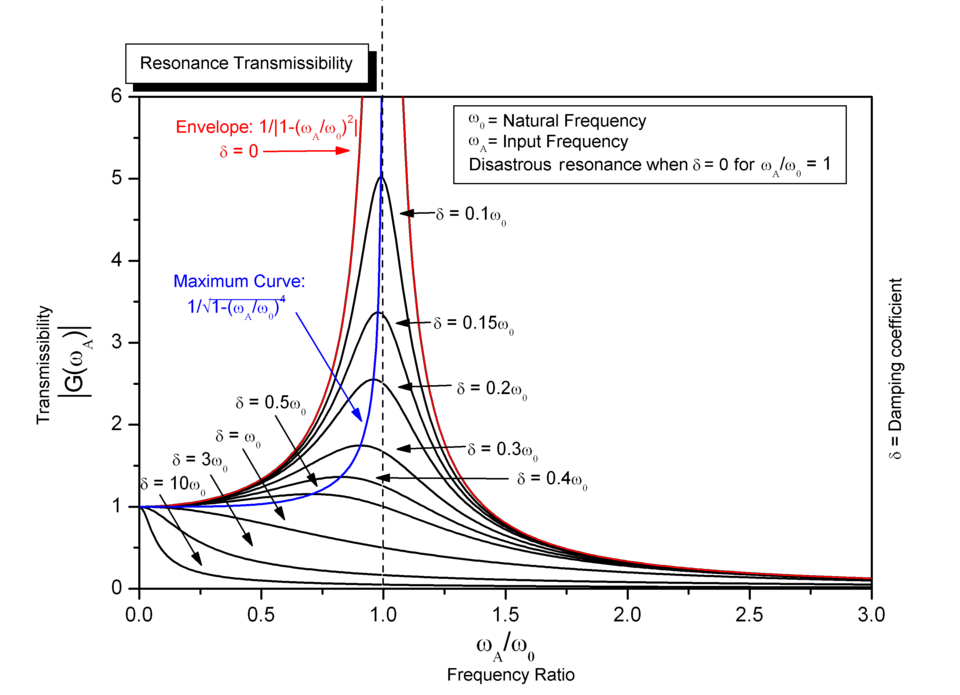
Graph showing resonance curves for different damping values, illustrating how lighter damping produces a tall, narrow peak while heavier damping produces a lower, broader peak. Extra annotations such as the envelope and maximum curve extend beyond OCR requirements but can be ignored. Source.
Damping: A resistive effect that dissipates energy from an oscillating system, reducing amplitude over time unless externally driven.
This means that the degree of damping directly controls how dramatic the resonance behaviour appears on the response graph.
Key damping effects on the graph:
Light damping
High maximum amplitude
Sharp, narrow resonance peak
Driving frequency at which maximum amplitude occurs is slightly below natural frequency
Heavy damping
Lower maximum amplitude
Broad resonance region
Peak shifts further below the natural frequency
A sentence must appear after these bullet points to maintain spacing between structural elements. These changes allow students to visually identify the level of damping in an oscillating system simply by examining the graph.
Interpreting Realistic Response Curves
To effectively interpret amplitude–frequency graphs, students should identify how amplitude varies across the range of driving frequencies and relate this variation to physical processes. They should also be familiar with how forced oscillators reach a steady-state amplitude, which is the constant amplitude observed after transient effects have died away.
Important interpretative steps include:
Observing whether the resonance peak is sharply defined or broad, indicating weak or strong damping respectively
Determining at which frequency the maximum amplitude occurs and comparing this with the known natural frequency
Noting the symmetry (or asymmetry) of the curve around the peak
Identifying how quickly amplitude falls off on either side of the resonance point
Recognising that the area under the curve does not represent energy but merely the system’s response pattern
A sentence is required here to separate structured elements: understanding these visual cues allows students to build correct conceptual links between theory and graphical representation.
Physical Interpretation of Resonance Behaviour
The height and sharpness of the resonance peak show how strongly the system responds to driving at different frequencies. The resonant amplification that occurs in low-damping conditions demonstrates how energy transfer from the external force into the oscillator is maximised at certain frequencies. The diminishing amplitude at higher or lower frequencies illustrates that the oscillator becomes increasingly out of phase with the driving force.
Resonance: A phenomenon in which a forced oscillator achieves maximum amplitude when the driving frequency is close to its natural frequency.
This definition is essential because resonance is at the centre of amplitude–frequency response analysis. The ability to relate resonance behaviour to the shape of the response curve is a core skill for interpreting these graphs.
Practical and Theoretical Insights
Amplitude–frequency response curves convey more than qualitative trends; they provide insight into how real systems respond under various forms of damping. Students examining these graphs should note the following interpretative principles:
Greater damping reduces overall system energy, lowering peak amplitude
Highly damped systems are less sensitive to variations in driving frequency
Lightly damped systems have pronounced frequency selectivity, showing strong resonance behaviour
The curve indicates how quickly an oscillator can respond to changes in driving frequency
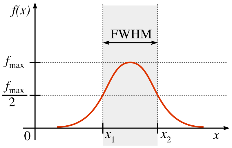
Resonance curve showing amplitude versus frequency with the bandwidth marked by the full width at half maximum (FWHM). The diagram illustrates peak sharpness, an indicator of damping strength. The explicit FWHM shading exceeds syllabus requirements but helps clarify why lightly damped systems display narrow resonance peaks. Source.
This final sentence ensures the structured sections remain properly separated while emphasising the analytical approach expected at A-Level.
Practice Questions
Question 1 (2 marks)
The amplitude of a forced oscillator is measured while the driving frequency is gradually increased. Describe how the amplitude changes as the driving frequency approaches and then exceeds the natural frequency of the oscillator.
Question 1 (2 marks)
1 mark: States that the amplitude increases as the driving frequency approaches the natural frequency.
1 mark: States that the amplitude decreases again once the driving frequency exceeds the natural frequency.
Question 2 (5 marks)
The graph below shows the amplitude–frequency response for two oscillators: one lightly damped and one heavily damped.
(a) Explain why the lightly damped oscillator has a sharper and higher resonance peak than the heavily damped oscillator.
(b) State two features of the amplitude–frequency response that allow you to identify which curve corresponds to the heavily damped oscillator.
Question 2 (5 marks)
(a)
1 mark: States that light damping means less energy is dissipated per cycle.
1 mark: States that the system stores more energy, leading to a larger steady-state amplitude at resonance.
1 mark: States that reduced damping results in a sharper (narrower) resonance peak.
(b)
1 mark: Identifies that the heavily damped oscillator has a lower maximum amplitude.
1 mark: Identifies that the heavily damped oscillator has a broader resonance region or peak shifted further below the natural frequency.
FAQ
The driving force continually adds energy to the oscillator at a rate that depends on how closely its frequency matches the system’s natural frequency. At steady state, the energy input each cycle balances the energy lost due to damping.
If the driving frequency is far from resonance, the oscillator responds weakly because the force is often out of phase with the motion. Near resonance, the force and displacement align more effectively, maximising energy transfer and producing a larger amplitude.
Damping introduces a resistive force that depends on velocity. This force alters the phase relationship between the driving force and the oscillator’s motion.
Because of this phase shift, the condition for maximum energy transfer no longer occurs exactly at the natural frequency. Instead, it occurs at a slightly lower frequency, with the shift becoming more pronounced as damping increases.
The width of the resonance peak, often referred to as the bandwidth, is directly linked to how quickly the oscillator dissipates energy.
A broader peak indicates:
Higher damping
Faster energy loss per cycle
Weaker frequency selectivity
A narrow peak corresponds to low damping, meaning the oscillator stores energy effectively and responds strongly only within a small frequency range.
At low driving frequencies, the oscillator moves almost in phase with the driving force. As the driving frequency increases towards resonance, the phase difference grows.
At resonance, the motion lags the force by roughly 90 degrees. Beyond resonance, the phase lag becomes greater than 90 degrees, approaching 180 degrees at very high frequencies. This progression strongly affects how efficiently energy is transferred at different frequencies.
Many real oscillators have additional complexities beyond ideal models, causing subtle distortions in their response curves.
Influencing factors include:
Non-linear restoring forces
Frequency-dependent damping
Structural variations or changing material properties
Interactions with surrounding media such as air resistance or fluid drag
These effects shift peak positions slightly, broaden specific regions of the curve, or create mild asymmetry while still following the core principles taught in the specification.
