Understanding exponential behaviour in capacitor circuits is essential for analysing charging and discharging; this section explores equations and how logarithm plots determine the time constant.

Exponential Behaviour in Capacitor Circuits

Exponential change is a defining characteristic of how capacitor charge, potential difference, and current vary when a capacitor is charged or discharged through a resistor. In the context of this subsubtopic, the focus is on applying exponential equations correctly and using natural logarithm (ln) plots to determine the time constant, RC, from experimental data. These mathematical tools allow precise interpretation of capacitor transients, which is vital for deeper analysis in electronics and circuit modelling.

When a capacitor is involved in a resistor–capacitor (RC) circuit, measurable quantities such as charge decrease exponentially during discharge and increase exponentially during charging. Understanding how these quantities evolve provides the foundation for predicting circuit behaviour and validating it through graphical methods.

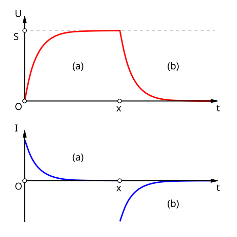
This figure shows the voltage and current in a capacitor–resistor circuit during both charging and discharging. The smooth curves illustrate the exponential approach to a final value on charging, and exponential decay towards zero on discharging. Minor extra annotations such as the saturation point simply emphasise the long-time behaviour and are not additional specification content. Source.

Exponential Equations for Discharging

One of the central exponential relationships is the equation describing how charge decreases during discharge. The quantity x may represent charge, current, or potential difference, depending on the measurement being analysed.

EQUATION
—-----------------------------------------------------------------
Exponential Decay (x) = x₀ e^(−t/RC)
x = The instantaneous value of the chosen quantity (C, A, or V)
x₀ = Initial value at t = 0 (same units as x)
t = Time elapsed (s)
R = Resistance controlling the discharge (Ω)
C = Capacitance of the capacitor (F)
—-----------------------------------------------------------------

During discharge, this equation predicts a continually decreasing value, approaching zero but never reaching it. This behaviour produces a smooth curve when plotted against time, and the gradient characteristics of this curve are essential when preparing data for an ln plot.

A key feature of exponential decay is that each equal interval of time results in the same fractional decrease of the quantity, which is directly linked to the mathematical form of the exponential function.

Exponential Equations for Charging

Charging a capacitor produces the opposite behaviour: the measured quantity rises towards a maximum value but never exceeds it. The relevant exponential relationship is given below and is essential for analysing charging graphs.

EQUATION
—-----------------------------------------------------------------
Exponential Growth (x) = x₀(1 − e^(−t/RC))
x = Instantaneous value during charging (C, A, or V)
x₀ = Final maximum value once fully charged (same units as x)
t = Time elapsed (s)
R = Circuit resistance (Ω)
C = Capacitance (F)
—-----------------------------------------------------------------

Although it represents growth rather than decay, this relationship includes the same exponential factor, e^(−t/RC), which ensures the shape retains the familiar flattening curve seen in capacitor-charging graphs.

Understanding both charging and discharging relationships deepens comprehension of Ln plots, because they ultimately rely on isolating the exponential term and expressing it in logarithmic form.

Preparing Data for Natural Logarithm Plots

Natural logarithm (ln) plots are used to transform a curved exponential graph into a straight line, allowing clear extraction of the time constant RC. This approach is valuable because it simplifies the experimental determination of RC, making it accessible even with simple measuring equipment.

To produce an ln plot from discharge data, the process typically follows these steps:

• Identify the measured quantity x (commonly potential difference across the capacitor).

• Apply the exponential decay equation.

• Rearrange to express ln(x) in terms of t.

• Plot ln(x) on the vertical axis and time t on the horizontal axis.

• Determine RC from the slope of the resulting straight line.

This method works because taking the natural logarithm of the exponential decay equation removes the exponential operator, leaving a linear relationship.

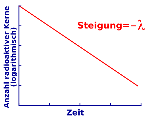
This logarithmic plot shows ln of an exponentially decaying quantity against time, producing a straight line with negative gradient. For a discharging capacitor, the vertical axis would represent ln(x), where x could be charge, voltage, or current, and the gradient would be −1/RC. Extra context in the original figure refers to nuclei and half-life, which is not required by the capacitor syllabus but follows the same exponential law. Source.

Deriving the Linear Form

To see how the exponential equation becomes linear, consider the decay relationship:

x = x₀ e^(−t/RC)

Taking the natural logarithm of both sides yields:

ln(x) = ln(x₀) − t/RC

This is the equation of a straight line of the form y = c + mx, where:

• y corresponds to ln(x)

• c corresponds to ln(x₀)

• m corresponds to −1/RC

The negative gradient is significant: it reflects the decreasing nature of the physical quantity during discharge.

The intercept ln(x₀) provides a useful check for data accuracy, as it should match the natural logarithm of the initial value obtained directly from the graph or measurement.

Interpreting the Gradient to Find RC

Once the ln(x) versus t graph has been plotted, its straight-line gradient is used to determine RC. Because the gradient equals −1/RC, extracting RC becomes straightforward by rearranging the relationship:

RC = −1 / gradient

This technique is highly valued in laboratory investigations because it mitigates the effect of small random fluctuations in the raw data. Instead of relying on individual points, the linear fit uses all data collectively to provide a reliable estimate.

Features of Successful ln Plots

To ensure validity when determining RC from experimental data, several conditions should be met:

• Measurements should be taken over a wide enough time range to capture the exponential trend clearly.

• ln(x) values should decrease in a regular, linear manner if the data are consistent with exponential decay.

• The straight-line fit should be assessed visually for uniformity; strong deviations may suggest experimental issues.

• The calculated gradient should be treated with attention to units, ensuring RC is ultimately expressed in seconds.

A secure understanding of these principles strengthens the ability to analyse capacitor circuits confidently and prepares students for more advanced treatments of transient electrical behaviour.