
OCR Specification focus:
‘Define half-life t₁/₂ = ln(2)/λ; describe experimental determination using suitable isotopes.’
Half-life is a concept describing the time taken for the activity or number of radioactive nuclei to fall by half, essential for understanding radioactive processes.
Half-life: Core Meaning and Importance
The half-life of a radioactive isotope is central to studying nuclear change and radioactivity. It provides a clear measure of how quickly unstable nuclei transform into more stable forms by emitting radiation. Because radioactive decay is spontaneous and random, the half-life offers a statistically reliable way to characterise the rate of decay without needing to predict individual nuclear events. The behaviour of large numbers of nuclei allows exponential laws to emerge, meaning half-life serves as a powerful tool for analysing nuclear processes in laboratories, medical applications, environmental studies, and industrial contexts.
Half-life (t₁/₂): The time required for the activity or number of undecayed nuclei in a radioactive sample to decrease to half its initial value.
Using half-life allows scientists to compare isotopes, identify suitable materials for particular experiments, and design detection methods appropriate to the radiation levels expected over time. It also enables practical work involving experimental measurement, where students are expected to handle data collection and interpret the decay behaviour of specific isotopes.
Mathematical Expression for Half-life
The OCR specification requires learners to recall and use the mathematical relationship connecting half-life and the decay constant. The decay constant λ quantifies the probability per unit time that an individual nucleus will decay. This probability remains constant even though the number of undecayed nuclei reduces over time.
EQUATION
—-----------------------------------------------------------------
Half-life (t₁/₂) = ln(2) / λ
t₁/₂ = Half-life in seconds (s)
λ = Decay constant in per second (s⁻¹)
—-----------------------------------------------------------------
This equation allows one to determine the half-life from knowledge of the decay constant, or vice versa, supporting further exploration of exponential decay behaviour. Understanding the relationship between λ and t₁/₂ is essential before attempting experimental measurement, as it provides the theoretical background against which results can be interpreted.
A radioactive sample always decays exponentially, meaning that the fraction lost per unit time is proportional to the number of atoms remaining. This characteristic ensures that even though the process is random on a nuclear scale, it becomes predictable when examining large numbers of nuclei.
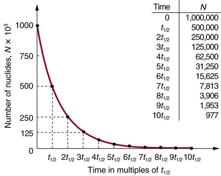
A graph of radioactive decay showing the quantity halving at regular intervals of t₁/₂. The curve illustrates exponential behaviour and the constant-probability nature of decay. This supports determining half-life from count-rate data by inspection or modelling. Source.
Experimental Determination of Half-life
The OCR syllabus specifically requires that students learn how to describe experimental determination of half-life using suitable isotopes. Such experiments must follow safe laboratory procedures, appropriate data collection methods, and careful interpretation of results. A typical setup involves detecting emitted radiation and monitoring how the measured count rate decreases over time.
Key Components of an Experimental Setup
Students must be familiar with the basic equipment used to monitor radioactive decay. Typical components include:
Radioactive source: Chosen for appropriate half-life length and safe handling requirements.
Detector (usually a Geiger–Müller tube): Produces count readings proportional to radiation intensity.
Counter or data logger: Records count rate at timed intervals.
Stable experimental arrangement: Ensures the distance between source and detector remains fixed and minimises background variation.
Shielding and safety equipment: Protects users from unnecessary exposure.
Because all radioactive measurements suffer from interference due to natural background radiation, background correction is essential for obtaining reliable values.
Procedure for Measuring Half-life
A clear, systematic approach is required to determine half-life experimentally:
Measure background count rate over several intervals to obtain a reliable average.
Place the radioactive source at a fixed distance from the detector.
Record count rate at regular time intervals, allowing enough time for clear decreases in activity to become measurable.
Subtract background count from each reading to obtain corrected activity values.
Plot corrected count rate against time to reveal the exponential decay trend.
Determine half-life either by identifying the time taken for activity to halve or by fitting an exponential curve to the data.
One complication arises when the half-life is very long or very short. Very long half-lives show activity changes too slowly for typical classroom timescales, while very short ones decay too quickly to record accurately without specialised equipment. This is why “suitable isotopes” are emphasised in the specification.
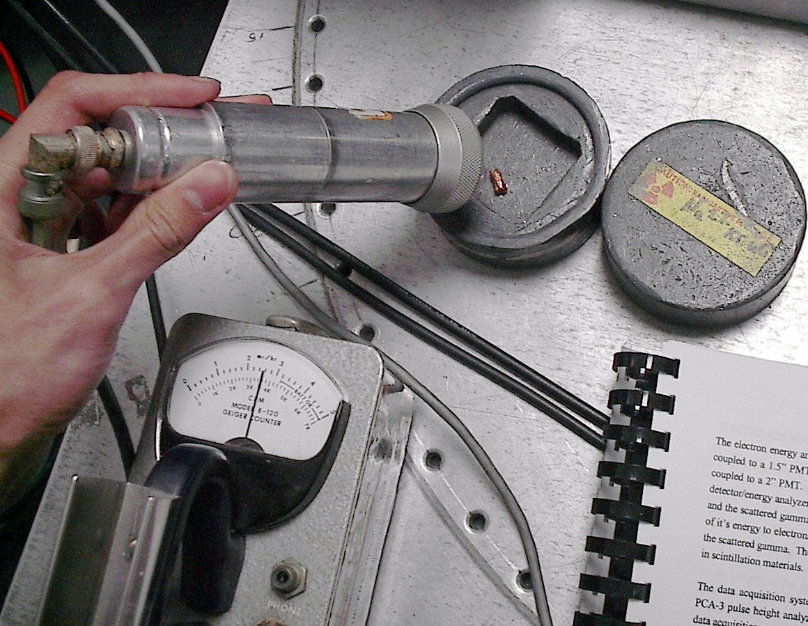
A laboratory arrangement demonstrating a Geiger–Müller counter with an end-window probe used to measure radiation from a sealed source. The fixed geometry supports accurate timed count measurements for half-life determination. Some additional accessories visible on the bench are standard but not required by the OCR specification. Source.
Characteristics of a Successful Measurement
Accurate experimental determination of half-life requires awareness of several important factors:
Consistency of timing is crucial. Using a stopwatch or data logger reduces human error.
Sufficient number of data points improves reliability when identifying halving times or fitting curves.
Stable detector response ensures systematic errors are minimised.
Appropriate choice of isotope allows measurable activity decrease within lesson duration.
Distance stability between the source and the detector avoids artificial variation in measured intensity.
Noise within radioactive data is expected because decay events are random. Even with careful measurement, count rates will fluctuate, yet the overall exponential trend becomes clear when plotted.
Interpretation of Results
Once data collection is complete, students should interpret the decay curve. For an exponential decay, each successive half-life shows the activity dropping by the same factor of two even though the absolute drop becomes smaller. Observing a smooth exponential decline indicates that the experiment has worked well and that background correction and timing procedures have been correctly applied.
Understanding half-life and its measurement ensures students can link theoretical decay laws to practical experimental techniques, fulfilling the requirements of the OCR specification for this subsubtopic.
Practice Questions
Question 1 (2 marks)
Define the term half-life and explain what is meant by saying that radioactive decay is random.
Mark scheme:
• Half-life is the time taken for the activity or number of undecayed nuclei to fall to half its initial value (1 mark).
• Radioactive decay is random because it is impossible to predict when any individual nucleus will decay (1 mark).
Question 2 (5 marks)
A student uses a Geiger–Müller tube to determine the half-life of a radioactive isotope that emits beta radiation.
They measure the background count rate, then record corrected count rates at regular time intervals and plot a graph of count rate against time.
(a) Explain why measuring and subtracting the background count rate is necessary.
(b) Describe how the student can use the plotted graph to determine the half-life of the isotope.
(c) State one experimental factor the student should keep constant during data collection and explain why.
Mark scheme:
(a)
• Background radiation contributes to the measured count rate (1 mark).
• Subtracting it ensures the count rate used represents only the decay of the source (1 mark).
(b)
• Identify the time interval during which the count rate falls to half its initial corrected value directly from the graph (1 mark).
• Alternatively accept using the exponential curve to find two points where activity halves and determining the time difference (1 mark).
(c)
• Keep the distance between the source and detector constant (1 mark).
• Because changing distance would change the count rate detected and distort the decay curve (1 mark).
FAQ
Half-lives vary because nuclear stability depends on the balance of forces within the nucleus. Some nuclei have configurations that make decay highly probable, while others are only very weakly unstable.
The likelihood of decay depends on factors such as nuclear binding energy, proton-to-neutron ratio, and available decay pathways.
As a result, half-lives can range from fractions of a second to billions of years.
Radioactive decay is unpredictable for any individual nucleus, but the behaviour of very large numbers of nuclei follows statistical laws.
Because the probability of decay per nucleus per second remains constant, the total number decaying per second becomes proportional to the number remaining.
This proportionality inevitably leads to an exponential decay curve.
Small timing inaccuracies can shift the plotted decay curve, making the halving point appear earlier or later than it should.
Timing errors may arise from:
• Delayed count recording
• Human reaction time
• Inconsistent interval spacing
• Equipment clock drift
Minimising these errors ensures the decay trend is measured reliably.
Short half-lives produce rapid activity changes that may be faster than the detector or data logger can measure.
Counts may fall too quickly, losing resolution.
Long half-lives produce activity changes so gradual that meaningful decay is not observable within a standard laboratory session.
This results in uncertainties larger than the decay itself.
Background radiation is not constant; it fluctuates depending on weather, altitude, building materials, and cosmic ray levels.
These fluctuations mean single background readings may not accurately represent the true average.
Taking several readings and finding a mean value reduces the impact of random variations and improves the reliability of corrected decay data.
