
OCR Specification focus:
‘Use A = A0 e^(−λt) and N = N0 e^(−λt); simulate decay with dice to illustrate randomness.’
Radioactive nuclei decay in a way that is inherently random yet statistically predictable, enabling physicists to model how the number of undecayed nuclei or activity changes with time using exponential relations.
Understanding Exponential Decay
Radioactive decay is a stochastic process, meaning that each individual nucleus decays unpredictably, but the overall behaviour of a large sample follows a consistent exponential pattern. This exponential trend allows physicists to relate the number of undecayed nuclei, the activity of a sample, and the decay constant, providing valuable tools for understanding and modelling nuclear behaviour.
When discussing exponential decay, the term activity appears frequently.
Activity: The rate at which nuclei decay in a radioactive sample, typically measured in becquerels (Bq), where 1 Bq = 1 decay per second.
The concept of decay constant is also crucial, as it directly determines the steepness of exponential decay.
Decay Constant (λ): The probability per unit time that a nucleus will decay.
These ideas underpin the exponential decay relationships used throughout A-Level Physics and the wider scientific community.
After these key ideas are introduced, it becomes easier to interpret how decay processes evolve with time.
Exponential Decay Equations
Two central exponential relations describe the change in a radioactive sample:
Number of Undecayed Nuclei
EQUATION
—-----------------------------------------------------------------
Number–Time Relation (N(t)) = N₀ e^(−λt)
N(t) = Number of undecayed nuclei at time t (no units)
N₀ = Initial number of undecayed nuclei (no units)
λ = Decay constant (s⁻¹)
t = Time elapsed (s)
—-----------------------------------------------------------------
This equation captures how the population of radioactive nuclei falls smoothly and predictably as time increases.
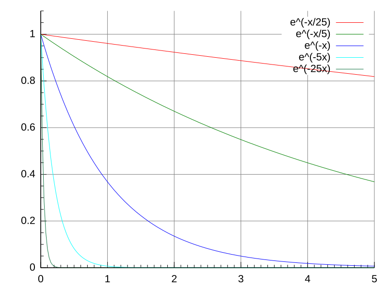
Exponential decay curves with different decay constants, showing how a larger λ produces a steeper decline. The vertical axis shows the remaining proportion, which asymptotically approaches zero. This visual directly reflects the mathematical form N(t) = N₀e⁻ˡᵗ and applies equally to activity due to proportionality. Source.
Activity of a Radioactive Sample
EQUATION
—-----------------------------------------------------------------
Activity–Time Relation (A(t)) = A₀ e^(−λt)
A(t) = Activity at time t (Bq)
A₀ = Initial activity (Bq)
λ = Decay constant (s⁻¹)
t = Time elapsed (s)
—-----------------------------------------------------------------
Because activity is directly proportional to the number of undecayed nuclei, both equations share identical mathematical form. Between these relations sits a simple proportional link:
A ∝ N.
Thus, any factor reducing the number of nuclei reduces the activity in exactly the same manner.
Interpreting the Decay Constant
The decay constant λ plays a central role in shaping the exponential curve. A large λ means nuclei have a high probability of decaying quickly, resulting in a steep drop in N and A. A small λ produces a shallower decay curve. The value of λ also connects directly to half-life through t1/2=ln2/λt_{1/2} = \ln 2 / λt1/2=ln2/λ, though the half-life relationship is not the main focus of this subsubtopic.
Research and technological fields use these exponential forms to predict how long radioactive materials remain hazardous or useful, reinforcing the relevance of λ in real scientific applications.
Graphical Behaviour of Exponential Decay
The exponential functions for both N(t) and A(t) create smooth, continuously decreasing curves with several key characteristics:
They decrease rapidly at first, especially for large values of λ.
They never reach zero, but asymptotically approach it over long timescales.
They allow for straight-line representation if plotted on a logarithmic scale, since ln(N) or ln(A) is proportional to −λt.
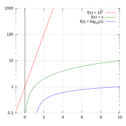
A semi-logarithmic graph in which the vertical axis is logarithmic and the horizontal axis is linear. Exponential relations appear as straight lines on such axes, making the decay constant observable from the gradient. The page also includes other plot types not required for OCR, but this log–linear form is the one relevant to radioactive decay. Source.
These graphical properties provide intuitive insights, making it easier for students to understand the long-term behaviour of radioactive substances.
Randomness and Dice Simulation
Although exponential decay equations describe the average behaviour of large samples, individual nuclei act randomly. To illustrate this, the OCR specification highlights using dice simulations.
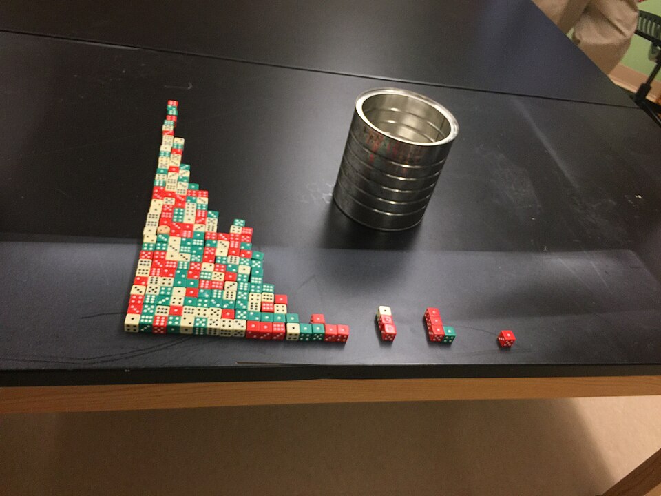
A classroom dice simulation representing radioactive nuclei, with each die acting as a nucleus that “decays” when a specific face is rolled. Removing decayed dice after each roll produces an approximately exponential decrease. The image includes surrounding lab context, but it remains fully aligned with the OCR-required decay simulation concept. Source.
A dice-based decay demonstration typically follows these ideas:
Treat each die as a single nucleus.
Assign a specific face (e.g., rolling a 1) to represent decay.
Roll the dice repeatedly; remove those “decayed” each round.
Count how many remain, forming an approximate exponential curve.
These simulations reinforce the statistical nature of decay:
Each nucleus has the same probability of decaying in each time step, just as each die has an equal chance of showing a particular face.
The decay of any individual nucleus cannot be predicted, but large populations behave predictably.
Repeating the simulation multiple times produces similar exponential trends, strengthening understanding of why the relation N = N₀e^(−λt) arises.
This conceptual tool bridges the gap between random microscopic behaviour and the smooth macroscopic decay equations used throughout physics.
Applying Exponential Relations
Students must be able to interpret and manipulate the exponential forms for N(t) and A(t) in qualitative contexts. Key applications include:
Recognising how a change in λ affects the steepness of decay.
Explaining why the same exponential form applies to both number of nuclei and activity.
Understanding how exponential behaviour reflects the constant decay probability of individual nuclei.
Interpreting decay curves on linear or logarithmic graphs.
These skills allow the exponential decay model to be applied widely in radiation physics, nuclear medicine, archaeology, environmental science, and reactor management.
In essence, exponential decay relations provide a compact yet powerful mathematical framework for describing radioactive processes, grounded in the combination of randomness at the nuclear scale and predictability at the population scale.
Practice Questions
Question 1 (2 marks)
Explain why the activity of a radioactive sample decreases exponentially with time.
Mark scheme:
• Each nucleus has a constant probability of decaying per unit time / constant decay constant. (1)
• Therefore the number of undecayed nuclei falls at a rate proportional to the number present, leading to exponential decrease in activity. (1)
Question 2 (5 marks)
A scientist models the decay of a radioactive isotope using the relation N = N0 e^(-lambda t).
(a) Describe the physical meaning of the decay constant lambda. (2 marks)
(b) Explain why a plot of ln(N) against time produces a straight line. (2 marks)
(c) State what the gradient of this line represents. (1 mark)
Mark scheme:
(a)
• Decay constant is the probability of a nucleus decaying per unit time. (1)
• A larger value of lambda means a faster rate of decay. (1)
(b)
• Taking natural logs of N = N0 e^(-lambda t) gives ln(N) = ln(N0) - lambda t. (1)
• This is in the form y = c + mx, so a straight-line relationship with time as the horizontal axis. (1)
(c)
• The gradient is equal to -lambda. (1)
FAQ
Exponential decay occurs when the rate of decrease is proportional to the quantity remaining, meaning the sample shrinks rapidly at first and then more slowly.
Linear decay would imply a fixed amount being lost per unit time, regardless of how much remains. This never occurs in radioactive decay because each nucleus has an independent and constant probability of decaying.
In an exponential process, the fraction lost per unit time stays constant, whereas in a linear process the absolute amount lost per unit time stays constant.
The mathematics of exponential functions means that the quantity asymptotically approaches zero but never becomes exactly zero.
Physically, this reflects the idea that although the probability of decay per nucleus is constant, there is always a non-zero chance that some nuclei may remain undecayed for very long times.
Only when all nuclei have individually decayed does the number become exactly zero, but the equation itself cannot predict the precise time this occurs.
Randomness affects each nucleus independently, but large samples display predictable statistical behaviour. This is a consequence of the law of large numbers.
When many nuclei are present, small fluctuations average out, producing a smooth decay curve.
Exponential relations arise because each nucleus behaves with the same constant probability per unit time, creating a stable pattern when scaled to millions or billions of nuclei.
Noise arises from detector limitations, counting statistics, and background radiation.
This can cause short-term fluctuations that deviate slightly from the ideal curve, especially when activity becomes very low.
To reduce such noise, experiments may:
• Take repeated measurements and average them
• Use shielding to reduce background counts
• Extend counting time intervals to smooth statistical variations
Radioactive decay spans large ranges of values, often decreasing by several orders of magnitude. A normal linear plot can compress later data into an indistinguishable region near zero.
A semi-log plot spreads out the values evenly by scaling the vertical axis logarithmically. This reveals trends that might otherwise be hidden.
It also linearises the exponential function, enabling easier determination of decay constants, half-life estimates, and comparison between different isotopes.
