
OCR Specification focus:
‘Model N(t) with spreadsheets and graphs; outline radioactive dating applications such as carbon dating.’
Graphical modelling allows physicists to visualise exponential radioactive decay, while dating techniques apply these principles to estimate the ages of materials. Both skills are essential for interpreting nuclear processes effectively.
Graphical Modelling of Radioactive Decay
Graphical modelling provides a powerful way to explore how the number of undecayed nuclei N(t) changes over time. Because radioactive decay is both random and spontaneous, graphs help reveal the smooth exponential trend underlying the statistical behaviour of large numbers of nuclei.
Exponential Decay Behaviour
Radioactive nuclei decay at a rate proportional to the number of nuclei remaining. This leads to an exponential decrease, and the key to understanding such behaviour is representing the decay law visually.
When first discussing the exponential decay equation, it is necessary to introduce the decay constant.
Decay Constant (λ): The probability per unit time that an individual nucleus will decay; measured in s⁻¹.
The exponential trend becomes clearer when plotting the number of nuclei or activity on a graph over time. Students are expected to use spreadsheet tools to model and visualise these relationships.
Between definition blocks, it is important to emphasise that spreadsheets generate data iteratively, reinforcing the link between probability and numerical decay sequences.
Form of the Exponential Decay Equation
For modelling, the fundamental decay equation is required.
EQUATION
—-----------------------------------------------------------------
Exponential Decay (N(t)) = N₀ e^(−λt)
N₀ = Initial number of nuclei (no unit)
N(t) = Number of nuclei at time t (no unit)
λ = Decay constant, probability of decay per second (s⁻¹)
t = Time elapsed (s)
—-----------------------------------------------------------------
Graphically, this produces a curve that rapidly falls at first and then gradually levels as fewer nuclei remain.
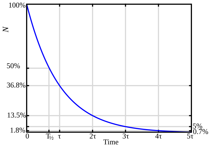
A labelled exponential-decay curve showing activity or nuclei number versus time, with the half-life indicated. The vertical axis is scaled to the percentage of the initial quantity, highlighting proportional decrease. This diagram directly represents the exponential trends students generate in spreadsheet modelling. Source.
The same mathematical structure applies to activity, because activity is proportional to the number of undecayed nuclei.
Normal text must separate equation blocks from other structural elements. The above equation forms the basis of all spreadsheet-generated decay graphs.
Using Spreadsheets to Model N(t)
Students are expected to model decay numerically using common spreadsheet software. Spreadsheets allow iterative recalculation of N(t) for small time increments, generating a smooth set of data points. To construct a practical model, students typically:
Create columns for time, decay constant, initial number of nuclei, and N(t).
Enter the exponential decay equation into spreadsheet cells so that each row computes the number of nuclei at a later time.
Use small time steps to approximate continuous decay.
Plot the resulting N(t) values as a graph to show the exponential trend.
Adjust λ or N₀ to observe how changing nuclear properties affects the decay curve.
This approach helps clarify the relationship between mathematical decay laws and physical radioactive processes. It also strengthens data-handling and computational skills relevant to A-Level Physics.
Graphical Interpretation Skills
Once plotted, decay graphs allow students to extract key physical insights. Important graphical features include:
Curve shape: Recognising an exponential form is essential for correctly interpreting nuclear decay.
Rate of decay: The steepness indicates how rapidly the nuclei disappear; steeper curves correspond to larger decay constants.
Half-life identification: The time interval for N(t) to fall to half its initial value can be read directly from the graph.
Long-term behaviour: Graphs illustrate that nuclei never reach zero instantaneously; the decay is continuous and smooth.
Spreadsheets also allow overlaying multiple decay curves—useful for comparing isotopes or contrasting theoretical and experimental data.
Radioactive Dating Applications
Graphical modelling underpins several scientific dating techniques. The OCR specification requires students to outline radioactive dating applications, particularly carbon dating, which relies on measuring the remaining proportion of radioactive isotopes in once-living material.
Principles of Radioactive Dating
Radioactive dating estimates the age of a substance by analysing how much of a specific radioactive isotope remains. The essential idea is that once a biological organism dies, it no longer exchanges carbon with the environment, so its proportion of radioactive carbon begins to fall according to the exponential decay law.
Radioactive Dating: The process of determining the age of a material by comparing the remaining quantity of a radioactive isotope to its expected initial amount.
This definition aligns closely with the principles observed in graphs of N(t), which show the reduction in nuclei over time.
Following this definition, we emphasise that dating techniques apply the same mathematical structure used in spreadsheet modelling.
Carbon Dating
Carbon-14 (¹⁴C) dating is the best-known application.
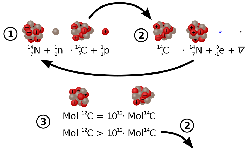
A diagram illustrating formation of ¹⁴C in the atmosphere and its subsequent decay to ¹⁴N used in radiocarbon dating. It reinforces how exponential decay governs the diminishing ¹⁴C content in once-living material. The inclusion of atmospheric formation pathways provides supportive context slightly beyond the OCR requirement. Source.
Living organisms maintain a nearly constant ratio of ¹⁴C to stable carbon isotopes through biological processes. After death, the ¹⁴C decays with a known half-life, so the remaining proportion indicates how long ago the organism died.
Key points about carbon dating include:
It relies on the exponential decay of ¹⁴C in organic remains.
Measuring the present activity or number of ¹⁴C nuclei allows estimation of elapsed time.
Graphs of N(t) help visualise how long half-life intervals correspond to measurable decreases in the isotope concentration.
Dating is reliable up to around fifty thousand years for carbon-based materials.
The technique supports research in archaeology, geology, and environmental science.
Graphical modelling helps students appreciate how the exponential decay curve connects directly to interpreting carbon dating measurements.
Wider Dating Applications
Other isotopes are used for extremely old rocks or geological samples. Though details vary, all such dating methods depend on:
Knowing the original quantity of the isotope (or using isotopic ratios).
Measuring current nuclei numbers or activities.
Applying the exponential decay relationship to estimate elapsed time.
Interpreting results through a decay curve similar to those generated in spreadsheets.
This reinforces the central idea that exponential decay graphs are not merely theoretical constructs but practical tools for determining the ages of materials across vast timescales.
Practice Questions
Question 1 (2 marks)
A student uses a spreadsheet to model the radioactive decay of an isotope by calculating values of N(t) at regular time intervals.
State two reasons why using a spreadsheet is useful for modelling exponential decay.
Mark scheme:
Award one mark for any two of the following, up to a maximum of 2 marks:
• Spreadsheet can rapidly calculate many values of N(t) for successive time intervals. (1)
• It automatically applies the exponential decay equation to each row, reducing error. (1)
• It allows easy plotting of a graph to show the exponential decay curve. (1)
• Parameters such as decay constant or initial number of nuclei can be changed to instantly update the model. (1)
Question 2 (5 marks)
Carbon-14 has a known half-life.
Describe how a scientist could use a graph of N(t) against time to estimate the age of an archaeological sample.
In your answer, refer to:
• how data for the sample would be obtained
• features of the decay curve
• how the graph is used to determine the age
• limitations of the method.
Mark scheme:
Award marks for the following points, up to a maximum of 5 marks:
• Measure the current activity or remaining proportion of carbon-14 in the sample. (1)
• Compare this measured value with typical initial activity/proportion for living organisms. (1)
• Plot or refer to a standard exponential decay graph of N(t) or activity against time for carbon-14. (1)
• Use the decay curve to find the time for the isotope to decay from the initial to the measured value. (1)
• Include at least one limitation, e.g. contamination, assumption of initial carbon-14 levels, or reduced accuracy for samples older than about 50 000 years. (1)
FAQ
A smaller time step makes the model more accurate because it approximates continuous decay more closely. Large time steps can cause noticeable numerical errors, especially early in the decay when the gradient is steep.
However, extremely small time steps increase the number of calculations and may introduce rounding errors in lower-precision software.
A balanced choice (for example, increments of a tenth or a hundredth of a half-life) is normally sufficient for OCR-level modelling.
The mathematical form of exponential decay approaches zero asymptotically, meaning it continually decreases without ever reaching zero on the curve.
In reality, nuclei decay one by one, and eventually none remain. The graph reflects the idealised mathematical model rather than the discrete nature of physical decay.
This distinction becomes important when interpreting long-term behaviour and understanding why very old samples may register extremely low but non-zero modelled values.
A clear decay graph should include:
• labelled axes with correct quantities and units
• a smooth exponential curve drawn from calculated data points
• a clearly marked initial value N0 or activity
• appropriate scaling so that early steep decay and later slow decay remain visible.
Adding gridlines or minor ticks can help students accurately identify the half-life or read intermediate values without altering the scientific content.
Uncertainties become proportionally larger as the sample becomes older, because activity approaches very low levels where measurement noise becomes significant.
Systematic effects also matter, such as detector efficiency or background radiation subtraction.
These uncertainties propagate through the decay equation, widening the possible range of ages and limiting the usefulness of carbon dating for extremely old samples.
Dating methods typically assume the initial proportion of the radioactive isotope is known or can be inferred from stable isotope ratios.
For carbon-14, it assumes living organisms share the same 14C/12C ratio as the atmosphere at the time.
If atmospheric composition varied, calibration curves must be applied to correct the graph-based age estimate, ensuring dates remain consistent across historical periods.
