
OCR Specification focus:
‘On displacement–time graphs, velocity equals the gradient; analyse linear and curved sections confidently.’
Understanding displacement–time graphs is fundamental to analysing motion. These graphs visually represent how an object’s position changes over time, allowing velocity and motion behaviour to be determined from the gradient.
Displacement–Time Graph Basics
A displacement–time graph shows how the displacement of an object changes with time. Displacement is a vector quantity, meaning it has both magnitude and direction, unlike distance, which is a scalar.
Displacement: The distance in a specified direction from an object’s initial position to its final position.
The horizontal axis of the graph represents time (t), while the vertical axis represents displacement (s). Each point on the graph corresponds to the displacement of the object at a particular time.
The shape and gradient of the line provide insights into how the object is moving:
A straight line indicates constant velocity.
A curved line indicates changing velocity (i.e. acceleration or deceleration).
Interpreting the Gradient: Velocity
The gradient (slope) of a displacement–time graph represents velocity.
This relationship is mathematically expressed as:
EQUATION
—-----------------------------------------------------------------
Velocity (v) = Change in displacement (Δs) ÷ Change in time (Δt)
v = Δs / Δt
v = velocity (m s⁻¹)
Δs = change in displacement (m)
Δt = change in time (s)
—-----------------------------------------------------------------
When the graph is a straight line, the gradient is constant, meaning velocity is constant. The steeper the gradient, the greater the magnitude of the velocity.
Between any two points on the graph:
The gradient = rise/run = (change in displacement) / (change in time).
A positive gradient means motion in the positive direction.
A negative gradient means motion in the opposite direction (returning towards the origin).
Linear Sections: Constant Velocity
Linear sections of a displacement–time graph correspond to uniform motion.
If the graph forms a straight line through the origin, the object moves with constant velocity and no acceleration.
Key points for interpreting linear sections:
Horizontal line (zero gradient): The object is stationary — displacement is not changing.
Upward sloping line: The object moves in the positive direction at constant velocity.
Downward sloping line: The object moves in the negative direction at constant velocity.
The slope’s numerical value directly represents the magnitude of the velocity, and its sign represents direction.
Curved Sections: Changing Velocity
Curved portions of a displacement–time graph indicate that the velocity is not constant — the object is either accelerating or decelerating. In these regions, the gradient changes continuously.
To interpret:
If the gradient increases over time, the object is accelerating.
If the gradient decreases over time, the object is decelerating.
At any point along a curve, the instantaneous velocity can be found by drawing a tangent to the curve at that point and calculating its gradient.
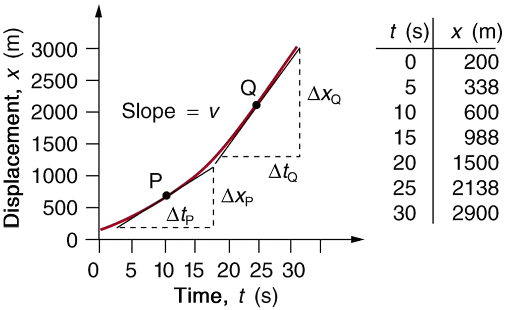
Displacement–time curve with tangents at two instants. The slope of each tangent gives the instantaneous velocity at that point. A steeper tangent indicates greater speed. Source.
Instantaneous Velocity: The velocity of an object at a specific moment in time, determined by the gradient of the tangent at that point on a displacement–time graph.
This distinction between instantaneous velocity (at a specific point) and average velocity (over a time interval) is crucial in motion analysis.
Analysing Gradients Step-by-Step
To confidently interpret displacement–time graphs, follow this process:
Identify linear or curved sections.
Straight lines represent constant velocity.
Curves indicate changing velocity.
Determine the direction of motion.
Positive slope → motion in positive direction.
Negative slope → motion in opposite direction.
Calculate gradients.
For straight lines, use two distinct points and compute rise/run.
For curves, draw a tangent and estimate its slope.
Link the gradient to physical meaning.
Constant gradient → constant velocity.
Increasing gradient → acceleration.
Decreasing gradient → deceleration.
Consider zero-gradient regions.
These indicate the object is momentarily at rest.
Each step ensures accurate physical interpretation aligned with the OCR requirement to analyse linear and curved sections confidently.
Non-Linear Motion Interpretation
When the motion involves variable acceleration (such as free fall with resistance or vehicle motion with changing power), displacement–time graphs often show complex curvature. Analysing these requires understanding how the gradient’s steepness changes.
Common features:
Concave-up curves (gradient increasing): the object accelerates.
Concave-down curves (gradient decreasing): the object decelerates.
Inflection points: points where acceleration changes sign, revealing transitions between speeding up and slowing down.
While precise quantitative analysis may require calculus (differentiating displacement with respect to time), at A-Level, qualitative understanding from the shape of the curve is sufficient.
Motion Direction and Reference Points
In real motion scenarios, the reference point (origin of displacement) must be defined.
Displacement can take positive or negative values, depending on the chosen coordinate system.
Key points:
A positive displacement means the object has moved away from the origin in the chosen positive direction.
A negative displacement means the object is on the opposite side of the origin.
The sign of the gradient (positive or negative) reflects direction of motion, not necessarily speed.
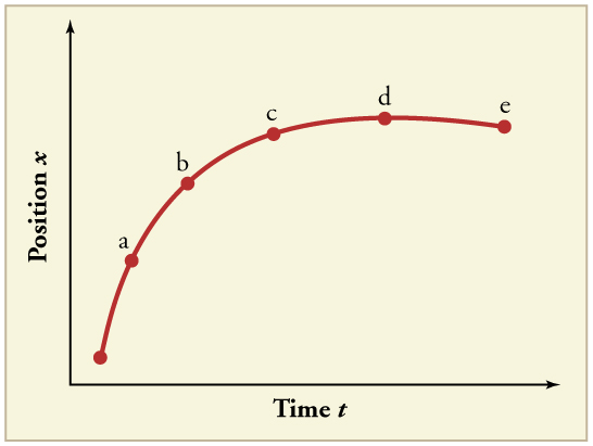
Position–time graph with multiple labelled points showing varying gradient. Positive slopes indicate motion in the positive direction, zero slope shows rest, and negative slope shows motion in the opposite direction. Source.
Velocity: The rate of change of displacement with respect to time, including both magnitude and direction.
In practical terms, the velocity–time graph derived from the gradient of a displacement–time graph allows for deeper motion analysis, such as calculating acceleration or total displacement in subsequent studies.
Key Observations for OCR Students
Displacement–time graphs are foundational tools for describing linear motion.
Velocity equals gradient, the central relationship of this subsubtopic.
Analysing linear sections confirms constant velocity.
Analysing curved sections reveals variable motion — acceleration or deceleration.
Tangent drawing is an essential skill for determining instantaneous velocity.
Students must interpret both magnitude and direction from graph gradients.
By mastering gradient analysis on both linear and curved displacement–time graphs, students gain the ability to interpret motion precisely, satisfying the OCR requirement to “analyse linear and curved sections confidently.”
Practice Questions
Question 1 (2 marks)
A student observes the motion of a trolley and plots a displacement–time graph. The graph shows a straight line passing through the origin with a constant positive gradient.
(a) What does the constant gradient of this displacement–time graph represent?
(b) What does the positive sign of the gradient indicate about the direction of motion?
Mark Scheme – Question 1
(a) Gradient represents velocity or speed in a particular direction. (1 mark)
(b) Positive gradient indicates motion in the positive direction or away from the origin. (1 mark)
Question 2 (5 marks)
A student analyses a displacement–time graph for a moving car. The graph shows a curve that becomes progressively steeper with time for the first 4 seconds and then a horizontal line for the next 2 seconds.
(a) Describe how the car’s velocity changes during the first 4 seconds.
(b) Explain what the horizontal section of the graph represents.
(c) Sketch or describe how the velocity–time graph would look for this motion.
(d) State how you could determine the instantaneous velocity at a specific time from the displacement–time graph.
Mark Scheme – Question 2
(a) Velocity increases because the gradient becomes steeper, meaning the car is accelerating. (1 mark)
(b) The horizontal section shows no change in displacement, so the car is stationary. (1 mark)
(c) Velocity–time graph would show an increasing line (upward sloping) during acceleration, followed by a flat line at zero velocity while stationary. (2 marks)
(d) Draw a tangent to the displacement–time curve at the required point and calculate its gradient to find instantaneous velocity. (1 mark)
FAQ
The slope of a displacement–time graph gives the velocity, which includes direction. A positive slope means motion in one direction, and a negative slope means motion in the opposite direction.
In contrast, the slope of a distance–time graph always gives the speed, which is a scalar quantity and cannot be negative. Therefore, distance–time graphs cannot show changes in direction, while displacement–time graphs can.
A curved graph shows that the gradient (velocity) is changing. When the steepness of the curve changes at a non-constant rate, the acceleration itself is changing.
This means the object experiences non-uniform acceleration, where:
Velocity increases or decreases unevenly over time.
The acceleration is not constant and could be due to variable forces such as air resistance.
When data points fluctuate due to measurement noise:
Draw a best-fit smooth curve through the data rather than joining points directly.
Find the gradient of the tangent to this smooth curve at the desired point.
Using digital tools such as data-logging software or spreadsheet smoothing functions can further reduce experimental error when estimating instantaneous velocity.
No. A vertical line would imply that displacement changes instantaneously while time remains constant, which is physically impossible.
All real motion must occur over a finite time interval. If a graph appears nearly vertical, it represents a very high velocity but not an instantaneous change.
A reversal in direction occurs when the gradient changes sign — from positive to negative or vice versa.
On the graph:
The line or curve reaches a maximum or minimum point (where the gradient is zero).
This point marks the momentary stop before the object moves in the opposite direction.
Such turning points are useful in analysing oscillations, projectile motion, or any movement involving back-and-forth motion.
