
OCR Specification focus:
‘Interpret spring force–extension graphs; identify linear regions, elastic limit and hysteresis where appropriate.’
Force–extension graphs reveal how materials respond to stretching forces, allowing analysis of elasticity, energy storage, and permanent deformation under increasing loads.
Understanding Force–Extension Relationships
A force–extension graph shows how the extension (increase in length) of a spring or material changes as an applied force increases. It visually represents Hooke’s law and helps determine key properties such as elasticity, stiffness, and energy storage.
Extension: The increase in length of a material when a tensile force is applied, calculated as the change between the stretched length and original length.
In these graphs, force is plotted on the vertical axis (y-axis) and extension on the horizontal axis (x-axis). The resulting curve provides direct insight into the mechanical behaviour of the material being tested.
The Linear (Proportional) Region
The linear region is the initial straight-line section of the graph where force and extension are directly proportional. In this region, the material obeys Hooke’s law, meaning that as the applied force doubles, the extension doubles as well.
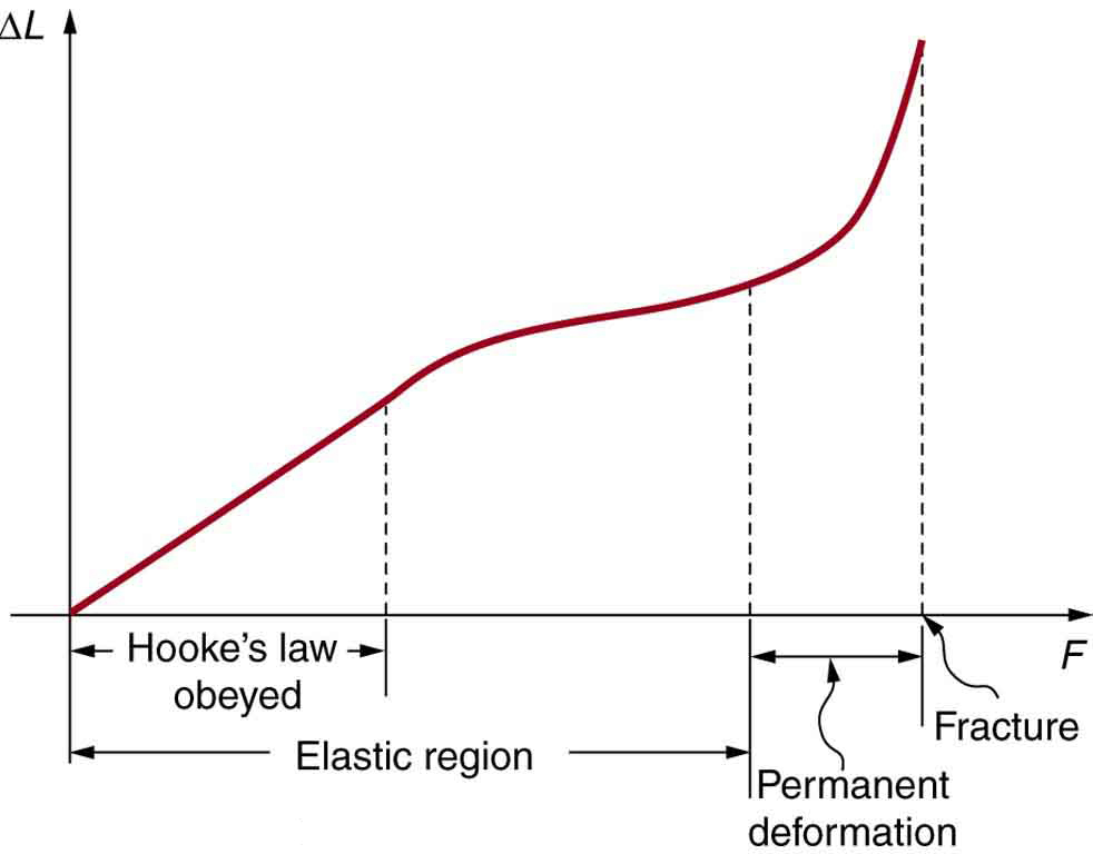
A deformation–force graph highlighting the Hooke’s law region (straight line), the wider elastic region, and the onset of permanent deformation leading to fracture. The figure helps students visually separate proportional behaviour from nonlinear elastic and plastic effects. The inclusion of “fracture” extends slightly beyond the OCR emphasis but clarifies the end of usable extension. Source.
EQUATION
—-----------------------------------------------------------------
Hooke’s Law (F = kx)
F = Force applied to the spring (N)
k = Force constant or spring constant (N m⁻¹)
x = Extension of the spring (m)
—-----------------------------------------------------------------
Within this linear region, the slope of the line gives the force constant (k), indicating the stiffness of the spring or material. A steeper slope means a stiffer material that requires more force to produce the same extension.
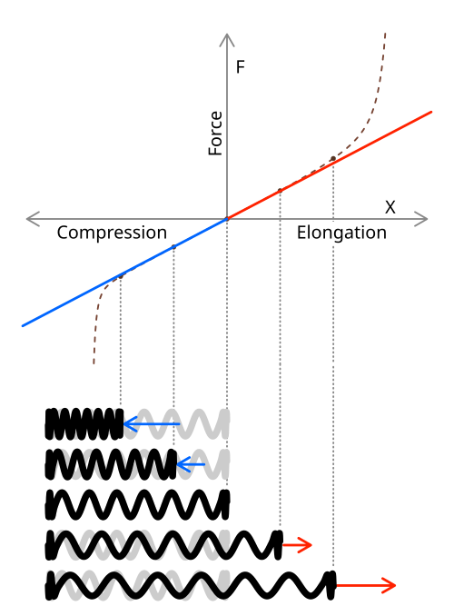
Force–extension plot for an ideal spring showing the linear Hooke’s-law region and a dashed non-ideal response at larger deformation where proportionality fails. The slope corresponds to the spring constant (k), so a steeper line indicates a stiffer spring. Small spring sketches link real spring states to positions on the graph. Source.
It is important to note that different materials or even identical springs of varying thicknesses can have different gradients, illustrating how structure affects stiffness.
The Limit of Proportionality
As force continues to increase, the graph eventually deviates from the straight line. The point where this deviation begins is known as the limit of proportionality.
Limit of Proportionality: The point beyond which force and extension are no longer directly proportional, and Hooke’s law ceases to apply.
Beyond this point, the extension increases more rapidly for a given increase in force, indicating that the material is undergoing non-linear elastic behaviour. Although the material may still return to its original length when the load is removed, the relationship is no longer proportional.
Elastic Limit and Elastic Deformation
At higher forces, the material reaches the elastic limit, a critical boundary distinguishing between elastic and plastic behaviour.
Elastic Limit: The maximum force or extension at which a material can be stretched and still return to its original shape when the force is removed.
Up to this limit, the deformation is elastic — all energy stored during stretching is recoverable. Beyond this limit, plastic deformation begins, meaning some deformation becomes permanent even when the force is removed.
In a force–extension graph, this transition typically appears as a curve flattening out beyond the linear region. For springs and most metals under low loads, this region is small, but for polymers or rubbers, it can be much more pronounced.
Beyond the Elastic Limit: Plastic Behaviour and Failure
When the applied force exceeds the elastic limit, the material enters the plastic region, where deformation is irreversible. The graph in this region curves progressively, showing that large extensions occur for relatively small increases in force.
Eventually, materials may neck or fracture, particularly in ductile metals or brittle materials such as glass. Although the OCR specification does not require detailed failure analysis here, recognising this region is useful for interpreting the limits of practical material performance.
Area Under the Graph: Work and Energy
The area under a force–extension graph represents the work done on the material during stretching. Up to the elastic limit, this energy is stored as elastic potential energy and is fully recoverable when the force is released.
EQUATION
—-----------------------------------------------------------------
Elastic Potential Energy (E = ½Fx or ½kx²)
E = Elastic potential energy stored (J)
F = Force applied (N)
x = Extension (m)
k = Spring constant (N m⁻¹)
—-----------------------------------------------------------------
While the relationship between force and extension remains linear, this area forms a right triangle under the line, making it straightforward to calculate energy. When non-linearity begins, the area can be determined by integration or approximation using the shape of the curve.
Hysteresis in Force–Extension Graphs
For certain materials such as rubber or polythene, the loading and unloading curves on a force–extension graph do not coincide.
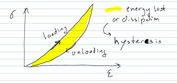
A loading–unloading curve illustrating hysteresis: the area between the two paths represents energy lost (e.g., as heat) during a stretch–relax cycle. This is typical of viscoelastic materials such as rubbers. The diagram is generic stress–strain, which maps directly to force–extension when geometry is fixed; no extra non-syllabus detail is included. Source.
This difference between the two paths forms a hysteresis loop.
Hysteresis: The phenomenon where the loading and unloading curves of a material differ, indicating energy loss (usually as heat) during deformation.
The area between the loading and unloading curves represents the energy dissipated as heat or internal friction. Unlike metals or springs that ideally return all energy elastically, these polymeric materials exhibit viscoelastic behaviour, combining both viscous (energy loss) and elastic (energy storage) properties.
Hysteresis is particularly significant in applications like rubber bands, vehicle tyres, and vibration dampers, where repeated loading and unloading occur.
Interpreting Features on a Force–Extension Graph
When analysing a typical spring or material force–extension graph, students should be able to:
Identify the linear region and apply Hooke’s law.
Mark the limit of proportionality where linearity ends.
Locate the elastic limit, beyond which permanent deformation occurs.
Recognise the plastic region, where deformation is irreversible.
Determine the area under the curve to find energy stored or lost.
Interpret hysteresis loops in materials exhibiting energy dissipation.
Each of these features provides insight into the mechanical behaviour of materials and their suitability for engineering or experimental use.
Practical Implications and Significance
Understanding force–extension graphs allows physicists and engineers to design materials and components that perform predictably under load. For example:
Springs in mechanical systems must remain within their elastic region for reliability.
Polymers with large hysteresis loops are valuable for energy absorption in damping applications.
Brittle materials, which show little plastic deformation, are suitable where rigidity is more important than flexibility.
By interpreting these graphs accurately, one can evaluate elastic properties, energy efficiency, and failure thresholds, all of which are central to the study of material behaviour under tension.
Practice Questions
Question 2 (5 marks)
A student investigates the behaviour of a spring by gradually increasing the applied force and measuring the extension. The resulting force–extension graph is shown to be straight initially, then curves and finally shows a small hysteresis loop when the load is removed.
(a) Explain what is meant by the linear (proportional) region of the force–extension graph. (2 marks)
(b) Identify and describe the significance of the limit of proportionality on this graph. (1 mark)
(c) Explain what the hysteresis loop represents and why it appears when the load is removed. (2 marks)
Mark scheme:
(a) Force and extension are directly proportional (1 mark). The spring obeys Hooke’s law and returns to its original length when unloaded (1 mark).
(b) The limit of proportionality is the point beyond which force and extension are no longer proportional / Hooke’s law no longer applies (1 mark).
(c) The hysteresis loop shows energy lost as heat or internal friction during loading and unloading (1 mark). It appears because the material is not perfectly elastic and exhibits energy dissipation (1 mark).
Question 1 (2 marks)
A student plots a force–extension graph for a metal spring and observes that the line is straight and passes through the origin.
(a) State the physical law demonstrated by this observation. (1 mark)
(b) Describe what this straight-line relationship indicates about the behaviour of the spring. (1 mark)
Mark scheme:
(a) Hooke’s law – 1 mark
(b) Force is directly proportional to extension / The spring obeys Hooke’s law within the elastic limit – 1 mark
FAQ
Several factors can affect how accurately a spring or material follows the theoretical linear relationship:
Measurement errors, such as parallax when reading the metre rule or misalignment of scales.
Temperature changes, which alter the spring’s stiffness by affecting the atomic bonding.
Uneven loading or bending, if the spring is not hung vertically or the force is not applied along its axis.
Material imperfections, like microcracks or uneven winding, which cause non-uniform stress distribution.
Minimising these factors ensures a more accurate determination of the linear region and spring constant.
The limit of proportionality marks where force and extension stop being directly proportional, while the elastic limit defines where permanent deformation begins.
A material can remain elastic (able to return to its original shape) even beyond the limit of proportionality, but the relationship between force and extension becomes non-linear.
In metals, these two points are often close together, but in polymers or rubbers, the difference is much greater due to molecular rearrangement before plastic deformation begins.
Plot a force–extension graph using measured data. In the linear region, the graph forms a straight line through the origin.
The gradient of this line equals k, the spring constant.
To increase accuracy, use multiple data points and calculate the gradient using a large portion of the line.
A steeper gradient indicates a stiffer spring.
If several springs are connected in series or parallel, their effective spring constant changes, but the determination method remains the same.
In a hysteresis loop, the loading curve represents energy supplied to stretch the material, while the unloading curve represents energy recovered.
The area between the two curves is energy lost as heat or internal friction within the material.
The area under the unloading curve alone shows the recoverable elastic energy. Materials with large hysteresis losses (like rubber) are ideal for damping and cushioning applications where energy absorption is beneficial.
Different atomic and molecular structures lead to characteristic force–extension curves:
Metals: Linear region up to the elastic limit, followed by a smooth plastic region before fracture.
Rubbers: Non-linear even at small forces, with significant hysteresis due to molecular chain movement.
Polythene strips: Show yielding and necking, with a pronounced non-linear shape.
These differences reflect how intermolecular forces and atomic bonds respond to applied stress, making force–extension graphs valuable for comparing material properties.
