Vector-valued functions let one parameter control several coordinates at once, making them a powerful way to represent curves, positions, and motion while still relying on familiar ideas from ordinary single-variable calculus.

What a Vector-Valued Function Is

A vector-valued function assigns a vector to each input value. In AP Calculus BC, the input is usually a parameter, often written as $t$. Each coordinate of the output is an ordinary real-valued function of that same parameter, so one input can determine an entire point in the plane or in space.

This means a vector-valued function packages several related real-valued functions into one object. Instead of listing coordinates separately, we can write them together in vector form. That notation is compact, but it also emphasizes that the coordinates describe one point moving as the parameter changes.

Component Functions and Notation

The coordinate functions inside a vector-valued function are called its component functions.

A common notation is $\mathbf{r}(t)$. In two dimensions, $\mathbf{r}(t)$ gives a point in the plane. In three dimensions, it gives a point in space. The domain of the function is the set of parameter values for which every component is defined.

In space, the same idea becomes $\mathbf{r}(t)=\langle x(t),y(t),z(t)\rangle$.

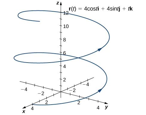
A space curve arises when the vector-valued function has three components, $\mathbf{r}(t)=\langle x(t),y(t),z(t)\rangle$. In this example, $\mathbf{r}(t)=\langle \cos t,\sin t,t\rangle$ produces a helix: the $x$–$y$ projection cycles around a circle while the $z$-coordinate increases steadily, creating a spiral in 3D. Source

The notation changes, but the principle stays the same: each coordinate is a real-valued function of the same parameter.

Connection to Parametric Equations

A vector-valued function in the plane is closely related to a pair of parametric equations. If $\mathbf{r}(t)=\langle x(t),y(t)\rangle$, then the same curve can be described by the coordinate equations $x=x(t)$ and $y=y(t)$.

Vector notation is useful because it keeps those coordinate functions connected. Rather than thinking of $x$ and $y$ as separate pieces, you view them as parts of one changing position. This is especially helpful when a problem describes a point moving along a curve or when three-dimensional motion is involved, because the same notation extends naturally to an added $z$-component.

A vector-valued function does more than describe where points lie. It also describes how the curve is traced as the parameter changes. Different parameter values may produce the same point, and the same geometric curve can sometimes be represented by more than one vector-valued function.

Domain and Geometric Meaning

The domain of a vector-valued function is found by checking where all component functions are defined at the same time. For example, if one component is defined for all real numbers and another is not, the overall domain is restricted by the component with the narrower domain.

The range is not just a set of numbers. It is a set of vectors, or equivalently, a set of points traced in the plane or in space. Geometrically, you can imagine the output vector starting at the origin and ending at the point determined by the component functions.

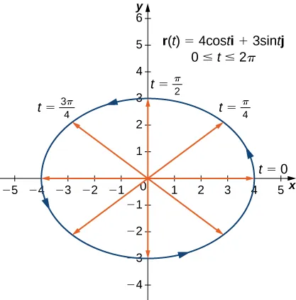
A planar vector-valued function $\mathbf{r}(t)=\langle x(t),y(t)\rangle$ can be visualized as a moving position vector whose tip traces a curve. Here, $\mathbf{r}(t)=\langle 4\cos t,3\sin t\rangle$ traces an ellipse, with arrows indicating the direction of increasing $t$ and labeled points showing specific parameter values. Source

As $t$ changes, the tip of that vector traces a curve.

Tracing a Curve

When you evaluate a vector-valued function at a specific parameter value, you substitute that value into each component. The result is one point on the curve. As the parameter increases, the point moves through the outputs in order. That order matters because it gives the curve an orientation, even when the graph itself looks familiar.

This interpretation makes vector-valued functions especially natural for describing motion. The parameter is often time, but it does not have to be. It can be any variable that controls position.

How Familiar Calculus Ideas Extend

The syllabus emphasizes that methods used for real-valued functions extend to vector-valued functions. The main reason is that each component is an ordinary function, so many ideas from single-variable calculus are applied component by component.

For an introduction, the most important extensions are conceptual:

• Evaluation: plug the parameter value into each component.

• Domain analysis: combine the restrictions from all components.

• Limits: a vector-valued function has a limit when each component approaches its own limit.

• Continuity: the function is continuous when all components are continuous.

These ideas do not require entirely new calculus rules. Instead, they rely on the same rules you already know for real-valued functions, used in a coordinated way. This is why vector-valued functions feel new in notation but familiar in method.

For AP Calculus BC, it is important to see that the vector notation does not replace the component functions; it organizes them. If you understand the behavior of the components, you can understand the behavior of the vector-valued function.

Common Interpretation Points

Students often confuse the function itself with the curve it traces. The function is the full rule $\mathbf{r}(t)$, including its parameter. The curve is the geometric path formed by the outputs. These are related, but they are not identical.

Another common issue is ignoring the parameter interval. A curve may be traced only partially if $t$ is restricted, or it may be traced more than once if the interval is large enough. Because of this, the parameter and its interval are part of the description, not just extra information.

Finally, remember that vector-valued functions are not limited to motion problems. They provide a general way to describe points changing together, and that makes them a bridge between algebraic functions, geometric curves, and later calculus operations.