For polar curves, second derivatives describe how a branch bends when viewed in rectangular coordinates. They are especially useful for determining concavity and for identifying points where the curve’s behavior changes.

What the second derivative tells you

A polar curve is given by an equation such as $r=f(\theta)$, but the second derivative $d^2y/dx^2$ still describes how $y$ changes with respect to $x$. This means you are studying the curve as it appears on the Cartesian plane, not just how the radius changes.

That distinction matters. A curve may have a simple polar equation and still produce complicated bending in rectangular form. For that reason, concavity for polar curves is determined from $d^2y/dx^2$, not from $d^2r/d\theta^2$.

When analyzing a polar curve, think of $\theta$ as the parameter tracing the curve. The same point in the plane can sometimes be reached by different values of $\theta$, so concavity must be interpreted along the specific branch being traced.

Building the formula

To find $d^2y/dx^2$, rewrite the polar curve in parametric form using $x=r\cos\theta$ and $y=r\sin\theta$.

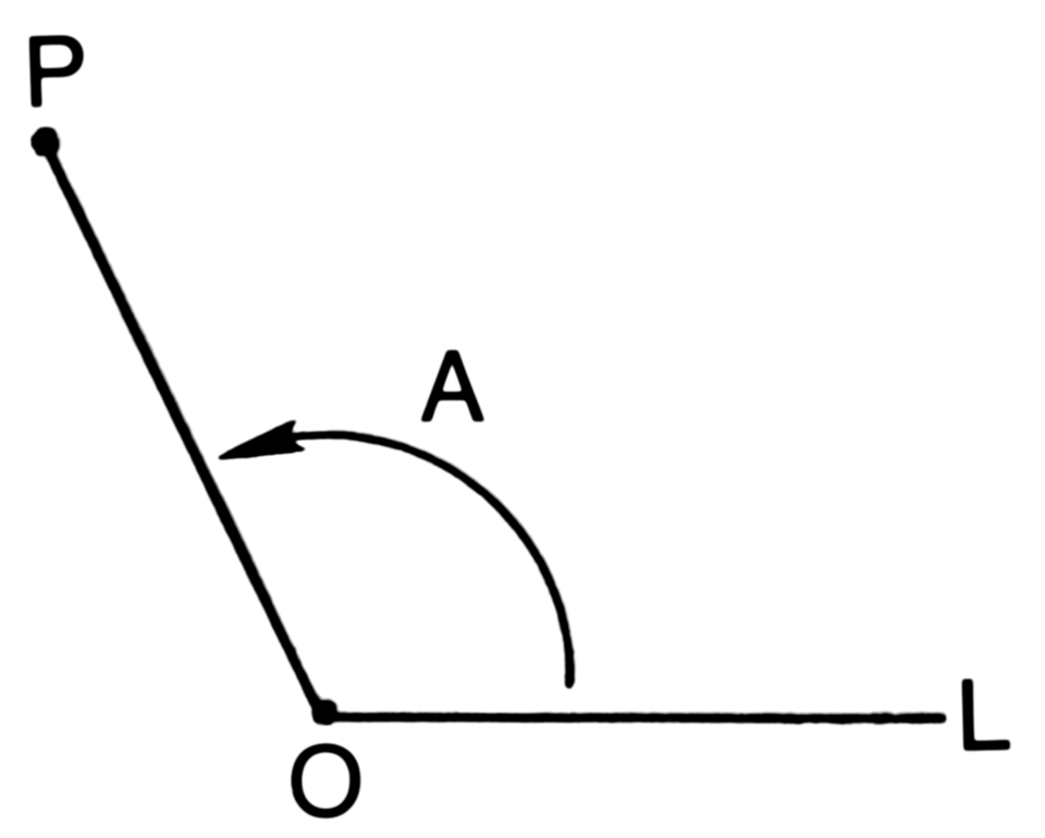
This diagram defines polar coordinates by showing a point $P$ located by a radial distance $r$ from the origin and an angle $\theta$ measured from the positive $x$-axis. It connects the geometric picture to the standard coordinate conversion formulas $x=r\cos\theta$ and $y=r\sin\theta$. Source

Then differentiate with respect to $\theta$.

This formula works when $dx/d\theta\neq 0$. For a polar curve, if $r'=dr/d\theta$, then

• $dx/d\theta=r'\cos\theta-r\sin\theta$

• $dy/d\theta=r'\sin\theta+r\cos\theta$

These expressions come directly from differentiating $x=r\cos\theta$ and $y=r\sin\theta$ with respect to $\theta$.

Once $dy/dx$ is known, differentiate it again with respect to $\theta$. That gives the rate at which the slope changes as the curve is traced. To convert that into a second derivative with respect to $x$, divide by $dx/d\theta$ again.

This is the polar version of the parametric second-derivative formula. It is the main tool for analyzing how a polar curve bends.

A reliable analysis process

When a problem asks about concavity or second-derivative behavior for a polar curve, use a consistent process:

• Start with the polar equation $r=f(\theta)$.

• Compute $r'$ if needed.

• Find $dx/d\theta$ and $dy/d\theta$ from $x=r\cos\theta$ and $y=r\sin\theta$.

• Form $dy/dx$ using $\dfrac{dy/d\theta}{dx/d\theta}$.

• Differentiate $dy/dx$ with respect to $\theta$.

• Divide by $dx/d\theta$ to get $d^2y/dx^2$.

• Determine where $d^2y/dx^2$ is positive, negative, zero, or undefined.

The sign of the second derivative gives the concavity of the traced branch over the interval of $\theta$ being considered. In AP Calculus BC, the interval matters because many polar curves are traced only on part of the full angle range, or they may retrace themselves.

Interpreting the result correctly

A positive value of $d^2y/dx^2$ means the branch bends upward as $x$ increases locally. A negative value means it bends downward. If the second derivative is zero, that alone does not guarantee an inflection point. You must check whether concavity actually changes.

There are several common issues to watch for:

When $dx/d\theta=0$

If $dx/d\theta=0$, the formula for both $dy/dx$ and $d^2y/dx^2$ can break down. This does not automatically mean the curve is discontinuous. It means the rectangular derivative test is not available in that form at that value of $\theta$.

When a point is traced more than once

A polar curve can pass through the same point for different values of $\theta$. In that situation, the curve may have different slopes or concavity on different branches. Always connect your second-derivative result to the specific interval of $\theta$ in the problem.

Near the pole

At points where $r=0$, the curve is at the pole. Polar curves often change direction rapidly there, and the second derivative may be difficult to interpret from the graph alone. Algebraic analysis is especially important.

Concavity is local

Concavity describes local bending, not the overall shape of the entire polar graph. A curve may switch between concave up and concave down several times as $\theta$ increases, even if it looks symmetric or familiar.

What AP questions usually expect

On AP Calculus BC, second-derivative analysis of polar curves usually involves these ideas:

• finding $d^2y/dx^2$ from a given $r=f(\theta)$

• deciding whether a branch is concave up or concave down

• identifying values of $\theta$ where concavity may change

• interpreting undefined second-derivative values carefully

The key idea is that polar curves are analyzed through their rectangular behavior. Even though the curve is given in terms of $r$ and $\theta$, the second derivative $d^2y/dx^2$ remains the standard test for concavity.