
AP Syllabus focus:
‘Exploring how calculators, standard normal tables, or computer-generated output can be utilized to find proportions of data within intervals of a normally distributed variable or to estimate population parameters.’
Using Technology to Analyze Normal Distributions
Technology plays a central role in AP Statistics by streamlining the process of working with normal distributions, enabling efficient computation of probabilities, areas under the curve, and estimates of unknown parameters.
Introduction
Modern statistical tools make analyzing normal distributions faster and more accurate, helping students compute proportions, evaluate intervals, and estimate parameters using reliable technological methods.
Understanding Technology in Normal Distribution Analysis
Technology helps overcome the limitations of manual calculation by providing quick access to areas under the normal curve, which are essential for determining proportions or probabilities.
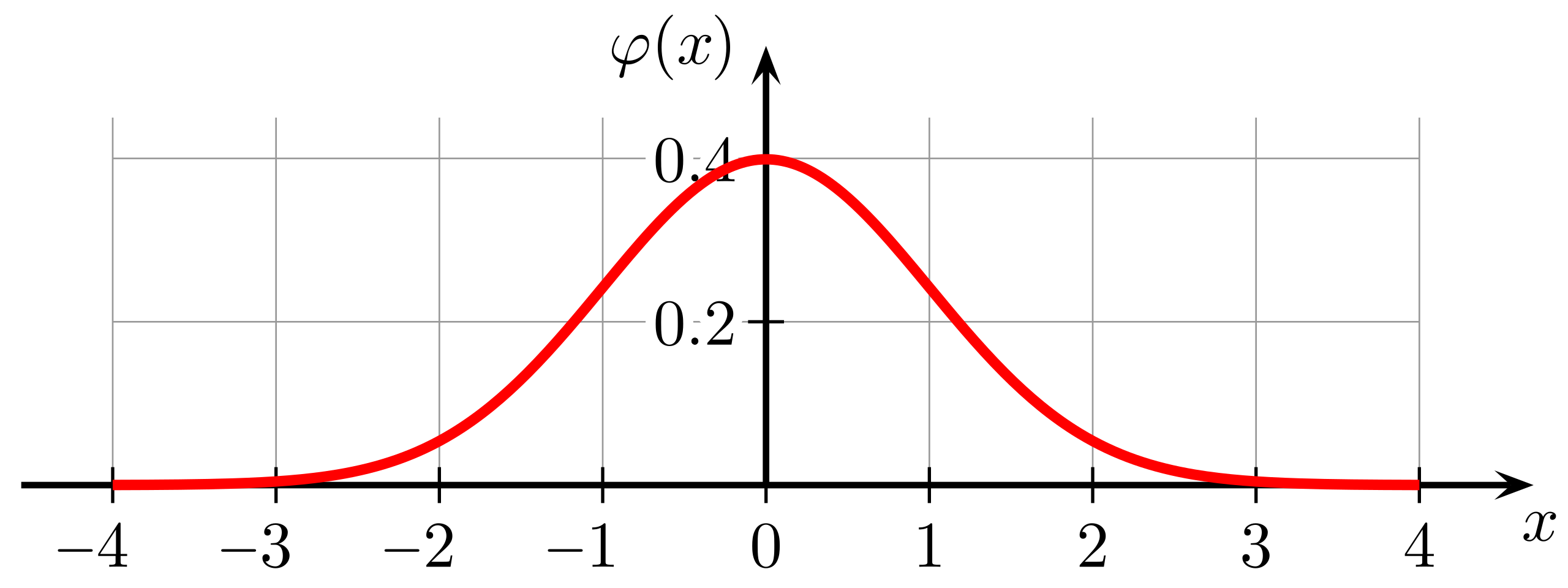
A smooth, symmetric bell-shaped curve represents the standard normal distribution used in many calculator and software functions. The horizontal axis shows standardized values (z-scores), while the vertical axis shows the corresponding probability density. This graph provides the foundation for interpreting areas under the curve as proportions of observations in a normally distributed variable. Source.
Whether using a graphing calculator, a standard normal table (also known as a z-table), or computer-generated output, the goal remains the same: to interpret normal models effectively and consistently.
The Role of the Standard Normal Distribution
The standard normal distribution is a special normal distribution with mean 0 and standard deviation 1. When technology performs a calculation involving a normal model, it typically converts data values into standardized units so that probabilities can be found using stored or built-in distribution functions.
Standard Normal Distribution: A normal distribution with mean 0 and standard deviation 1, used as a reference for finding probabilities and proportions.
Graphing calculators and statistical software access programmed algorithms that evaluate areas using the cumulative distribution function, or CDF, which gives the probability of observing a value less than or equal to a given point.
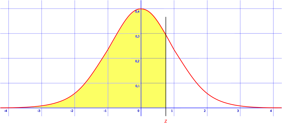
The shaded region under the standard normal curve shows the cumulative probability from negative infinity up to a particular z-value. This area corresponds to the output of a CDF or NormalCDF command on a calculator or in software. The curve emphasizes that as the cutoff value increases, the cumulative probability approaches 1. Source.
Using Calculators for Normal Distribution Calculations
Graphing calculators such as the TI-83/84 include built-in commands designed specifically for analyzing normal distributions. These tools allow students to determine proportions of observations falling within one or more intervals. When a calculator computes these values, it uses numerical methods to approximate the exact area under the continuous curve.
Key Calculator Functions
Most devices provide at least two essential functions:
A normal cumulative distribution feature for finding probabilities based on bounds.
An inverse normal feature for locating values corresponding to specific percentiles.
When technology uses these functions, it relies on the normal probability model and the parameters mean and standard deviation, which define the shape and spread of the distribution.
EQUATION
NormalCDF(lower, upper, μ, σ) = proportion in interval
μ = mean of the normal distribution
σ = standard deviation of the normal distribution
Students should understand that changing the bounds or parameters alters the area returned, reflecting different interpretations within real-world contexts.
Standard Normal Tables as a Technological Tool
Although digital tools are prevalent, the standard normal table still functions as an important form of technology.
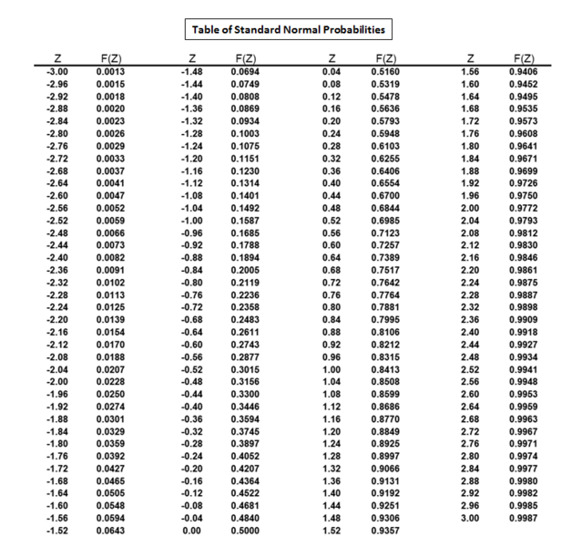
This standard normal table lists cumulative probabilities for a range of z-scores, with the row and column headings indicating the z-value and the body entries giving the corresponding area to the left. Students can use it to find proportions or critical values when modeling data with a standard normal distribution. The table includes more z-values than are typically needed in an AP Statistics context, but its structure is standard across textbooks and exams. Source.
These tables store cumulative probabilities associated with z-scores and allow users to locate proportions by scanning row and column combinations. This structured reference provides the same information that calculators compute, though it requires manual lookup and interpretation.
Z-Table: A tabular display listing cumulative probabilities for z-scores in the standard normal distribution.
Standard normal tables reinforce students’ understanding of how probabilities relate to standardized positions, supporting learning even when more advanced tools are used.
Computer-Generated Output and Statistical Software
Statistical software packages and online tools provide additional support by generating precise numerical outputs and graphs. These programs can display probability density curves, shade regions under the curve, and compute associated areas. They may also estimate population parameters when given sample data and assumptions of normality.
Computer-generated output often includes values such as the mean, standard deviation, and cumulative probabilities. These automated features allow students to interpret results without performing tedious integrations or calculations.
Benefits of Software-Based Analysis
Students gain:
Rapid computation of areas within complex intervals.
Visual displays that reinforce conceptual understanding.
Access to more precise probability values than those found in printed tables.
Tools for estimating parameters under normally distributed conditions.
Estimating Population Parameters Using Technology
Technology supports parameter estimation by processing sample data and producing estimates based on normal distribution assumptions. When a computer or calculator analyzes data from a population believed to follow a normal model, it can approximate unknown values such as the true mean or standard deviation.
EQUATION
μ-hat = sample mean
σ-hat = sample standard deviation
These estimates are essential inputs when technology is later used to compute probabilities or percentiles for the same population. After determining the estimated parameters, software tools apply built-in normal distribution functions to deliver probability-based interpretations.
Integrating Technology into Statistical Thinking
Understanding how calculators, tables, and software operate helps students interpret their computational results with greater confidence. Technology enhances accuracy, reduces computational errors, and supports the AP Statistics emphasis on interpreting contextually meaningful information drawn from normal distribution models.
FAQ
A suitable calculator should include built-in functions for cumulative normal probabilities and inverse normal calculations. These allow you to compute proportions and percentile values efficiently.
It is also helpful if the calculator provides graphing capabilities, as visualising the curve and shaded regions can reinforce conceptual understanding.
Many students use devices with a statistical distribution menu, ensuring easy access to normal distribution tools without navigating complex settings.
Technology typically produces values with greater precision because it calculates probabilities algorithmically rather than relying on rounded table entries.
While the two methods are broadly consistent, tables often round to four decimal places, whereas calculators may give six or more, leading to slight differences in the final probability.
These discrepancies are acceptable in examination conditions, provided the method used is clear and consistent.
Some tools assume you are working directly with the standard normal distribution, so they expect z-scores rather than raw data.
Others allow you to enter the mean and standard deviation of the original distribution, automatically converting values into standardised units internally.
Always check whether the interface refers to z, mean, or standard deviation to ensure correct interpretation of the output.
Before relying on technology to estimate parameters using normal models, confirm that the dataset appears reasonably symmetric and mound-shaped.
Check for:
• Clear absence of extreme outliers
• A single, dominant mode
• No strong skewness
These conditions make normal-based estimates more trustworthy and prevent misleading conclusions.
Density values correspond to the height of the normal curve at a specific point, while cumulative values represent the area to the left of that point.
Software includes both because density helps with visual interpretation of the distribution’s shape, whereas cumulative values are needed for probability-based reasoning.
This dual output allows users to analyse how the curve behaves at a point while simultaneously interpreting probabilities across intervals.
Practice Questions
A study reports that the heights of adult males are normally distributed with mean 178 cm and standard deviation 7 cm. Using technology, determine the proportion of adult males taller than 190 cm.
Correct use of technology-supported normal calculation: NormalCDF(190, large value, 178, 7) or equivalent (1 mark).
Correct proportion stated (approximately 0.080 or 8.0%) (1 mark).
Total: 2 marks.
A manufacturing process produces metal rods whose lengths are modelled by a normal distribution with mean 52.4 mm and standard deviation 1.3 mm.
A company inspector uses a calculator’s NormalCDF function to analyse production quality.
(a) Use technology to determine the proportion of rods shorter than 50 mm.
(b) The longest 5% of rods are considered oversized. Use appropriate technology to estimate the minimum length a rod must have to be classified as oversized.
(c) Explain why using technology is especially useful for these probability and percentile calculations.
(a)
Correct use of technology: NormalCDF(negative large value, 50, 52.4, 1.3) (1 mark).
Correct probability (approximately 0.020 or 2.0%) (1 mark).
(b)
Recognition that the 95th percentile is required (1 mark).
Correct use of inverse normal technology: InvNorm(0.95, 52.4, 1.3) or equivalent (1 mark).
Correct approximate value (about 54.5 mm) (1 mark).
(c)
Clear explanation that technology avoids manual integration or complex table lookups and provides more accurate probability/percentile estimates (1 mark).
Total: 6 marks.
