
AP Syllabus focus:
‘Understanding the importance of graphical representations and statistical summaries in highlighting key features of data.
Learning to represent categorical data using frequency tables, which list the number of cases for each category.
Exploring how to use relative frequency tables to provide the proportion (or percentage) of cases falling into each category, offering a comparative view of category sizes.
Skill 2.B: Developing proficiency in constructing and interpreting frequency and relative frequency tables for categorical data.
Essential Knowledge UNC-1.A.1: Mastery of frequency and relative frequency tables, including their creation and purpose.’
This section introduces two essential tools for organizing categorical information, emphasizing how structured summaries help reveal patterns, highlight differences between categories, and support meaningful interpretation of data.
Understanding Categorical Data and the Purpose of Tables
Categorical data consist of observations classified into distinct groups, such as types, labels, or qualitative characteristics. Because these groups do not follow a numerical scale, frequency and relative frequency tables provide the foundational methods for summarizing how many observations fall into each category. They play a critical role in highlighting key features of data, as required by the specification, by transforming raw observations into structured summaries that are easy to interpret. Students must demonstrate Skill 2.B, which includes constructing and interpreting these tables accurately and consistently in context.
Frequency Tables
A frequency table organizes categorical data by listing all observed categories alongside the number of observations belonging to each category. The purpose is to create a clear count-based summary that captures the distribution of the variable.
Frequency Table: A structured display showing each category in a dataset and the number of observations (counts) that fall within that category.
A frequency table is essential because it transforms scattered observations into an organized format, enabling quick identification of dominant categories, rare categories, and overall distribution shape.
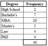
This frequency table summarizes CEO degree categories and their corresponding counts, illustrating how categorical data are organized into a clear, structured display. Source.
Components of a Frequency Table
A well-constructed frequency table typically contains:
Category labels, listed clearly and without overlap
Frequencies (counts) for each category
Total sample size, connecting individual counts to the broader dataset
These components allow students to remain attentive to context, a fundamental requirement noted in UNC-1.A.1.
Relative Frequency Tables
A relative frequency table extends the frequency table by expressing each category’s count as a proportion or percentage of the total number of observations. This representation provides a comparative view of category sizes, enabling meaningful comparisons even across samples of different sizes.
Relative Frequency Table: A table showing each category and the proportion or percentage of the total sample that falls within that category.
While a frequency table describes how often each category appears, a relative frequency table communicates how large each category is relative to the entire dataset, making it particularly useful for comparing categories in context.
A sentence here is necessary before any equation box is presented to maintain the required formatting structure.
EQUATION
= Number of observations in the category
= Sum of counts across all categories
Relative frequencies are indispensable when interpreting data in terms of proportions, and they are required knowledge under Essential Knowledge UNC-1.A.1.
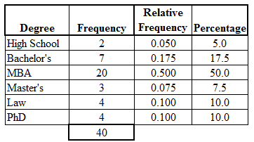
This expanded table demonstrates how each frequency value is converted into a relative frequency and a percentage, illustrating the construction of relative frequency tables from basic counts. Source.
Constructing Frequency and Relative Frequency Tables
Students develop proficiency by following a systematic process. Clear steps ensure accuracy and reinforce conceptual understanding.
Step 1: Identify All Categories
Before constructing any table, list all distinct groups present in the dataset. This step prevents omissions and maintains a consistent structure for analysis.
Step 2: Count the Frequency of Each Category
Once categories are identified, tally the number of observations falling into each one. Counting must be performed carefully, especially in large or unordered datasets.
Step 3: Compile the Frequency Table
Place each category and its associated count into a clearly organized layout.
Bullet-point organization ensures clarity:
List categories in a logical order (alphabetical, numerical, or contextual)
Align counts directly with the appropriate category
Verify that the sum of frequencies matches the total sample size
Step 4: Calculate Relative Frequencies
Divide each category’s count by the total sample size to determine the proportion or percentage.
Key reminders:
All relative frequencies combined should sum to approximately 1 (or 100%)
Round proportions or percentages consistently
Step 5: Interpret the Tables in Context
Interpreting tables requires students to focus on patterns, comparisons, and dominant categories, aligning with the specification’s emphasis on understanding how statistical summaries support insight. Students should:
Identify the most and least common categories
Compare relative sizes among categories
Connect findings to the real-world context of the dataset
Why These Tables Matter in Statistical Analysis
Frequency and relative frequency tables form the backbone of early data analysis. They support more advanced graphical representations such as bar charts and segmented bar graphs, and they prepare students for deeper interpretive tasks. By mastering these tables, students gain the ability to distill large sets of categorical information into meaningful summaries, meeting both Skill 2.B and the conceptual expectations of the AP Statistics curriculum.
FAQ
A frequency table groups identical categories together, allowing you to see the structure of the data at a glance rather than scanning through every individual item.
It also ensures:
No category is overlooked
Counts are consistent
Data can be compared or converted into other forms (such as relative frequencies)
Relative frequencies standardise the data so that category sizes are expressed as proportions of the whole rather than absolute numbers.
This means two datasets can be compared even if one is much larger, as differences reflect genuine tendencies rather than sample size effects.
A frequency table should include all categories present in the dataset, but categories may be combined if:
The original categories are too detailed
Two categories are nearly identical
Combining them produces clearer or more meaningful summaries
However, combining categories must be justified and should not distort the data’s meaning.
There is no fixed rule, but common approaches include:
Alphabetical order
Order of appearance in the raw data
Increasing or decreasing frequency
A logical or contextual order (e.g., small to large, early to late)
The chosen order should make the table easier to interpret.
Percentages are often easier for readers to interpret quickly, especially for non-specialist audiences.
Percentages also:
Make small differences more visible
Allow clearer comparisons between categories
Match how information is commonly presented in reports and media
Practice Questions
A supermarket records the type of fruit purchased by 120 customers. Explain what is meant by a frequency table when representing this categorical data.
(2 marks)
States that a frequency table lists categories and shows how many observations fall into each category. (1)
Refers to organising categorical data into counts to summarise the distribution. (1)
A school surveys 200 students about their preferred method of travel to school: walking, cycling, bus, or car.
(a) Construct a frequency table and a relative frequency table using the following data:
Walking: 50 students
Cycling: 30 students
Bus: 70 students
Car: 50 students
(b) Explain how the relative frequencies help in comparing the popularity of travel methods among the students.
(5 marks)
(a)
Correctly lists the four categories. (1)
Correctly assigns the given frequencies to each category. (1)
Calculates the correct relative frequency for each category (Walking 0.25, Cycling 0.15, Bus 0.35, Car 0.25). Award 1 mark for two correct values, 2 marks for all correct. (2)
(b)
Explains that relative frequencies show the proportion of the total for each category, allowing comparison regardless of sample size. (1)
States that they make it easier to compare popularity by expressing results on a common scale. (1)
