
AP Syllabus focus:
‘Explaining stem and leaf plots, including their structure where data values are divided into a "stem" and a "leaf". Demonstrating how stem and leaf plots provide a clear view of the data's distribution while retaining the actual data values for reference. Skill 2.B: Gaining proficiency in constructing and analyzing stem and leaf plots to visualize quantitative data distributions.’
Stem and leaf plots offer a compact, information-rich way to display quantitative data while preserving individual values, enabling students to visualize distribution shape and identify key features efficiently.
Understanding the Purpose of Stem and Leaf Plots
A stem and leaf plot is a graphical representation used to display the distribution of a quantitative variable, presenting data in an ordered, interpretable form without losing individual observations. These plots allow viewers to see patterns such as clusters, gaps, and outliers, while simultaneously retaining the raw numerical values. This dual function supports statistical reasoning by combining graphical overview with data-level detail.
Structure of a Stem and Leaf Plot
The defining feature of a stem and leaf plot is its division of each data value into two components: a stem, containing all but the final digit, and a leaf, containing the final digit.
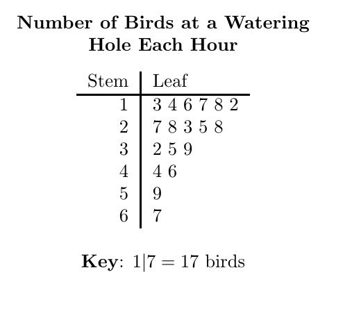
A stem and leaf plot displaying the number of birds observed at a watering hole each hour, clearly separating stems from leaves to demonstrate how individual values are preserved. Source.
Stem: The part of a quantitative data value containing every digit except the final digit.
A stem typically represents place-value structure, such as tens or hundreds, depending on the scale of the dataset. This organizational design groups related values together, making patterns easier to observe.
Leaf: The final digit of a quantitative data value, placed to the right of its corresponding stem.
Each row of the plot consists of a stem followed by one or more leaves, with leaves usually arranged in ascending numerical order within a row. This ordering allows the plot to function similarly to a sorted list, while still conveying distributional features visually.
A stem and leaf plot differs from other graphs because it preserves actual values rather than summarizing them into bins or intervals. This preservation provides a detailed look at the spread and frequency of observations.
Constructing a Stem and Leaf Plot
Creating a clear and readable stem and leaf plot involves a consistent process that aligns with the AP Statistics expectation of Skill 2.B, emphasizing accuracy and interpretability.
Steps to Construct
List all data values and determine the appropriate place-value division between stems and leaves.
Identify the range of stems needed by finding the smallest and largest stems.
Write each stem in a vertical column, ensuring the sequence follows numerical order.
Assign each data value to its correct stem by recording only the leaf digit beside that stem.
Order the leaves on each row from smallest to largest to clarify distributional patterns.
Title the plot and, when necessary, provide a key explaining how to interpret the digits (e.g., “4 | 7 means 47”).
These steps support uniformity and help ensure that the resulting plot accurately reflects the data’s structure.
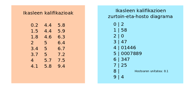
Caption: A stemplot displayed beside the original data values used to construct it, illustrating how ordering and grouping data points form a readable stem and leaf plot. Source.
Interpreting Stem and Leaf Plots
Once constructed, a stem and leaf plot becomes a powerful tool for analyzing the distribution of a quantitative variable.

A stem and leaf plot of prime numbers less than 100, demonstrating how stems represent tens digits and leaves represent ones digits to reveal patterns across value groups. Source.
Because the display maintains raw data values, students can inspect both the overall pattern and the precise observations simultaneously.
Key Features to Observe
Shape: Determine if the data appear symmetric, skewed, unimodal, or multimodal by examining how leaves cluster across stems.
Center: Approximate a middle value by identifying the location where leaves balance across the plot.
Variability: Evaluate how spread out the leaves are along the sequence of stems.
Unusual features: Look for gaps (stems with no leaves), clusters (densely populated stems), or unusually high or low values.
A stem and leaf plot is particularly effective for small to moderate-sized datasets because it balances visual clarity with informational detail. Although other graphs, such as histograms or dotplots, provide strong summaries, stem and leaf plots uniquely display each value explicitly, supporting richer interpretation.
Variations and Extensions
While the basic form is widely used, several variations help adapt the stem and leaf plot to different types of quantitative data.
Common Extensions
Split stems: Used when many leaves appear on a single stem, increasing readability by dividing each stem into two or more sub-stems (e.g., one for leaves 0–4 and another for 5–9).
Back-to-back plots: Place two sets of leaves on opposite sides of a shared stem, enabling direct comparison of two related datasets.
Truncated or rounded leaves: Apply when values have more digits than can be easily represented, provided rounding rules are used consistently.
Each variation maintains the fundamental requirement of retaining actual data values while enhancing the clarity of the distributional display.
Why Stem and Leaf Plots Matter in AP Statistics
This subsubtopic emphasizes constructing and analyzing stem and leaf plots because they reinforce students’ skills in reading, organizing, and interpreting quantitative data. The structure directly supports understanding of distributional features, aligning with the AP focus on graphical reasoning. Additionally, because the plot keeps raw data visible, it provides a foundation for later analyses involving shape, center, and variability, helping students transition into more advanced statistical representations.
FAQ
Choosing the stem–leaf split depends on how detailed you want the plot to appear and how large the data values are.
If values have many digits, you may need to use more than one digit for the stem to keep the plot readable.
If the leaves become too numerous on a single stem, consider splitting stems or adjusting the place-value cut.
A useful guideline:
• Aim for stems that create between 5 and 15 rows to maintain clarity and interpretability.
Split stems are helpful when a single stem has too many leaves, making the plot crowded.
To apply them:
• Divide each stem into two or more sub-stems (commonly 0–4 and 5–9).
• Ensure consistency across all stems so the distribution remains comparable.
Split stems reveal patterns that may be hidden in more compressed plots, such as subtle clustering or the presence of mid-range values.
Yes, stem and leaf plots can display decimal values effectively.
Place the decimal within the stem or leaf depending on convenience. For example, values like 3.4, 3.7 and 4.2 could use stems for whole numbers and leaves for tenths digits.
Alternatively, multiply all values by 10 to convert them into whole numbers before plotting and include a note explaining the scaling.
This makes the plot easier to read while preserving meaningful precision.
Unlike grouped tables, stem and leaf plots retain every individual value. This avoids losing detail when data are compressed into intervals.
They allow you to:
• Identify local clusters and isolated values.
• Detect subtle gaps within ranges that grouped tables may obscure.
• Access original measurements for further calculations without referring back to raw data.
This is especially useful for small datasets where fine detail matters.
A back-to-back plot places one set of leaves to the left of the stems and the other to the right, allowing direct comparison of distributions.
Ensure:
• Both datasets use identical stems and the same place-value rules.
• Leaves are ordered outward from the stem for clarity.
This format highlights contrasts in clustering, spread and central tendency without converting data into separate graphs or tables.
Practice Questions
Question 1 (3 marks)
A set of quantitative measurements is displayed using a stem and leaf plot.
(a) State what the ‘stem’ represents in a stem and leaf plot.
(b) State what the ‘leaf’ represents.
(c) Explain one advantage of using a stem and leaf plot instead of a simple ordered list of data.
Question 1
(a) 1 mark:
• Stem is all digits of a data value except the final digit.
(b) 1 mark:
• Leaf is the final digit of the data value.
(c) 1 mark (any one of the following):
• Shows distribution shape while preserving actual values.
• Easier to identify clusters, gaps or outliers than in a list.
• Provides both ordered data and a graphical overview simultaneously.
Question 2 (5 marks)
A physics student records a series of time intervals (in seconds) for a repeated reaction-time experiment and decides to represent the data using a stem and leaf plot.
(a) Describe the steps required to construct a clear and accurate stem and leaf plot from the raw data.
(b) Explain how the completed stem and leaf plot can be used to comment on the distribution of the time intervals.
(c) Suggest one reason why a stem and leaf plot may be particularly useful for small sets of measured physical data.
Question 2
(a) Up to 2 marks (any two of the following):
• Identify appropriate place-value split for stems and leaves.
• List stems in numerical order.
• Place each data value on the correct stem as a leaf.
• Order leaves on each stem from smallest to largest.
• Include a key explaining how to read the plot.
(b) Up to 2 marks (any two of the following):
• Identify features such as symmetry, skewness, clusters or gaps.
• Comment on the spread of values indicated by the range of stems and leaves.
• Identify unusually high or low time intervals.
(c) 1 mark:
• Because it preserves individual measured values while still showing overall distribution, which is useful for small datasets.
