
AP Syllabus focus:
‘Explanation of quartiles (Q1 and Q3) and their significance in representing the boundaries for the middle 50% of values in an ordered data set.
- Describing the calculation of the pth percentile as the value below which a certain percent of observations fall.
- Skill 2.C: Developing proficiency in determining quartiles and percentiles for quantitative data and understanding their application.’
Quartiles and percentiles help describe how data values are positioned within an ordered dataset, allowing statisticians to interpret distribution structure, locate relative standing, and summarize variability.
Understanding Position Within an Ordered Dataset
Quartiles and percentiles are measures of relative position, meaning they describe where a value lies within a distribution rather than summarizing all values at once. Because they rely on the order of data, they provide insight into how spread out observations are and how individual values compare to the dataset as a whole. These concepts are foundational for understanding the structure of the middle 50% of data, identifying boundaries between sections of the distribution, and assessing concentration patterns.
The Role of Quartiles
Quartiles divide an ordered dataset into four equal parts, creating three cut points that mark important distribution landmarks. The focus in AP Statistics is on Q1 (first quartile) and Q3 (third quartile), which enclose the central portion of the data and support further summary measures such as the interquartile range.
Quartile: A numerical boundary that divides ordered data into four equal sections, marking 25%, 50%, and 75% positions within the distribution.
Quartiles are essential in describing the spread and clustering of observations, especially when identifying where the middle half of the data lies and how separated or compact those values appear.
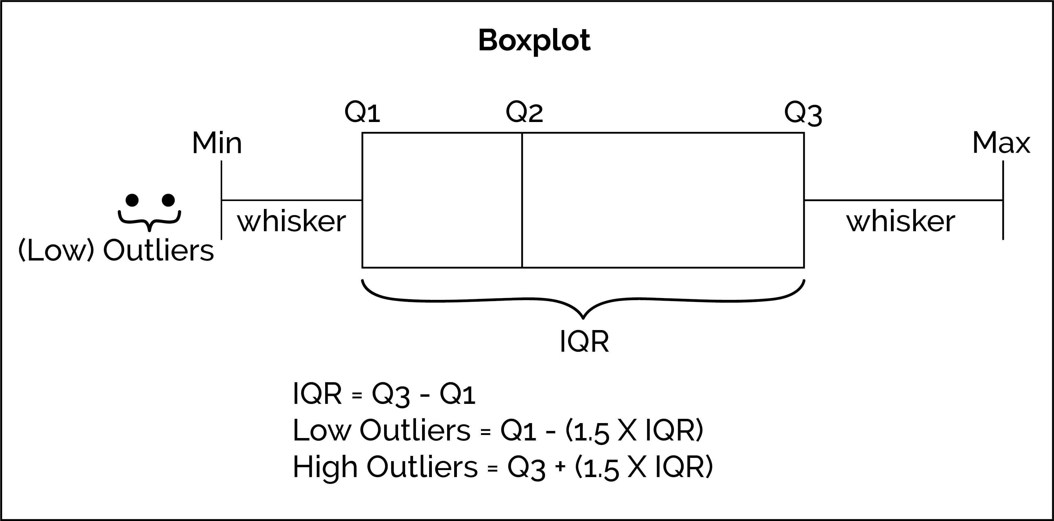
This diagram shows a horizontal boxplot with Q1, median (Q2), and Q3 labeled, along with whiskers and the interquartile range (IQR). It reinforces how quartiles divide ordered data into four equal parts and how the box highlights the middle 50% of observations. The formulas for outlier fences extend beyond this subsubtopic and can be ignored here. Source.
Understanding Q1 and Q3
Q1 (first quartile) identifies the value below which 25% of observations fall, while Q3 (third quartile) identifies the value below which 75% of observations fall. These two boundaries frame the middle 50%, known as the interquartile region, which is less influenced by extreme values than full-range measures.
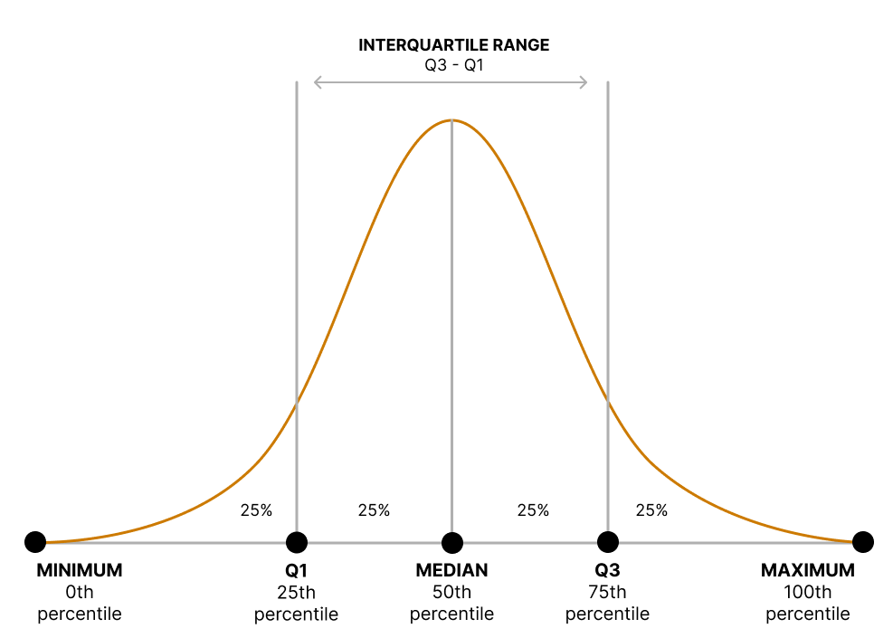
This figure shows a bell-shaped distribution annotated with the minimum, 25th percentile (Q1), median, 75th percentile (Q3), and maximum, with an arrow marking the interquartile range. It emphasizes how Q1 and Q3 bound the middle half of the data while linking quartiles to percentiles. The minimum and maximum extend slightly beyond this subsubtopic but remain consistent with context. Source.
Interquartile Region: The middle half of a dataset, bounded by Q1 and Q3, representing where typical or central observations are most concentrated.
These boundaries help determine not only the structure of the dataset but also the degree of variability within its central portion. Understanding their placement supports meaningful comparisons between groups and contributes to justified interpretations of distribution shape and spread.
Percentiles and Their Interpretive Value
Percentiles extend the idea of quartiles by dividing the dataset into 100 equal parts. The pth percentile identifies a value below which p percent of observations fall. Percentiles allow for finely tuned positioning of data and make it possible to describe standing relative to the entire dataset with more detail than quartiles alone.
Percentile: A measure indicating the value below which a specified percentage of observations in an ordered dataset fall.
Percentiles are widely used in fields such as education, health, and environmental studies because they allow for intuitive interpretation of rank or standing. They communicate both relative performance and the distributional structure that contributes to such interpretations.
Calculating Quartiles
Determining Q1 and Q3 requires ordering data from smallest to largest and locating the values that correspond to the 25th and 75th percent positions. AP Statistics emphasizes understanding the conceptual meaning of these cut points, regardless of small procedural variations in calculation methods. The essential idea is to determine boundaries that separate the dataset into proportional sections.
EQUATION
= Positions marking boundaries of the middle 50% of data
Quartiles support identifying skewness, examining concentration, and analyzing patterns that are not immediately visible from raw data alone.
A normal explanatory sentence is required here to maintain flow between equation blocks, reinforcing that these measures function as anchors for understanding distribution shape and central spread.
Calculating the pth Percentile
Percentile calculation also begins with ordering the data, then determining the value associated with the targeted percentage. Because percentiles provide a continuous scale of positional measures, they can describe standing with greater precision than quartiles and support interpretations for any selected percentage.
EQUATION
= Chosen percent identifying proportion of observations below the value
Percentiles and quartiles work together to deepen understanding of distribution structure, allowing students to describe data relative to proportional positions rather than individual values. The AP focus ensures that students interpret these measures correctly, emphasizing context, conceptual accuracy, and appropriate application in describing quantitative variables.
FAQ
Different methods vary in how they split the data when the median lies between values. Some include the median in both halves, while others exclude it.
These differences generally lead to small changes in Q1 and Q3, especially in small data sets. For large data sets, the methods produce nearly identical results.
When interpreting quartiles, exam questions expect consistency within the chosen method rather than a universally “correct” value.
Quartiles represent positions in an ordered data set, not necessarily actual data points.
When the calculated position lands between two values, the quartile is defined as the midpoint between them.
This ensures quartiles accurately mark the proportional locations (25 per cent and 75 per cent) even when the data set size does not align perfectly with these percentages.
Yes, quartiles and percentiles can provide clues about skewness by comparing distances between them.
For example:
• If Q3 is much further from the median than Q1, the distribution may be right skewed.
• If Q1 is further from the median than Q3, the distribution may be left skewed.
These indications are not definitive but offer a useful preliminary assessment when only summary measures are available.
Percentiles allow comparison across unrelated data sets because they measure relative position rather than actual values.
For example, a student in the 90th percentile in one exam and the 85th in another performed better relative to their peers in the first exam, even if the tests used different scales.
This makes percentiles helpful in contexts such as admissions, fitness assessments, and standardised testing.
In small samples, multiple values may occupy the same percentile boundary because ordering does not always create unique percentile locations.
In such cases:
• The percentile is still defined by its positional rule.
• Any tied values at that position legitimately represent the percentile.
• Interpretation focuses on the proportion of data, not the uniqueness of the value.
This is a normal feature of discrete, limited sample sizes and does not indicate an error in calculation.
Practice Questions
Question 1 (1–3 marks)
A data set of 40 ordered values has a 25th percentile of 18.4.
(a) State what this percentile value means in the context of the data set.
(b) Explain whether the 25th percentile is the same as the first quartile.
Question 1
(a) 1 mark: Correct interpretation that 25 per cent of the observations are less than or equal to 18.4, or that 18.4 marks the value below which a quarter of the data lie.
(b) 1 mark: States that the 25th percentile is the same as the first quartile.
1 additional mark (optional depending on wording): Brief explanation that the first quartile corresponds to the point separating the lowest 25 per cent of ordered observations.
Question 2 (4–6 marks)
A researcher collects 32 observations on the time (in minutes) students spend revising each day. After ordering the data, the researcher identifies that the 8th value is 22 minutes, the 16th value is 35 minutes, and the 24th value is 47 minutes.
(a) Determine the positions of the first quartile and the third quartile in this data set and identify their corresponding values.
(b) Using your answers to part (a), describe the spread of the middle 50 per cent of revision times.
(c) The researcher claims that most students revise for about the same amount of time each day. Use the quartiles to comment on whether this claim is supported.
Question 2
(a)
• 1 mark: Identifies the position of Q1 as the 8th value.
• 1 mark: Identifies the position of Q3 as the 24th value.
• 1 mark: States Q1 = 22 minutes and Q3 = 47 minutes.
(b)
• 1 mark: States that the middle 50 per cent of revision times lie between 22 and 47 minutes.
• 1 mark: May additionally describe IQR = 25 minutes (not required but creditworthy if stated correctly).
(c)
• 1 mark: Comments meaningfully on the researcher’s claim using quartiles, e.g., “The wide interval between Q1 and Q3 shows that revision times vary substantially, so the claim that most students revise for about the same amount of time is not well supported.”
• 1 mark: Reasoning clearly tied to the magnitude of the middle 50 per cent or the spread between quartiles.
