
AP Syllabus focus:
‘Utilizing summary statistics represented graphically (e.g., through boxplots) to make justified claims about the data in context. Discussing the relationship between distribution symmetry and the relative positions of mean and median, including implications for skewness (right or left). Skill 2.A: Enhancing proficiency in describing and interpreting graphical representations of summary statistics to support data analysis and conclusions.’
A understanding of graphical summary statistics helps students interpret distributions effectively, connecting numerical measures to visual patterns that support clear, context-driven conclusions in data analysis.
Describing Summary Statistics Graphically
Graphical displays of summary statistics translate numerical information into visual form, allowing patterns in a quantitative distribution to be recognized quickly. When summary statistics such as the five-number summary, median, or measures of center and spread are presented graphically—most commonly through boxplots—they become accessible tools for identifying distributional features and making justified statements about data within context. Effective interpretation requires careful attention to how each graphical element corresponds to numerical values.
Graphical forms such as boxplots visually encode essential distribution characteristics.
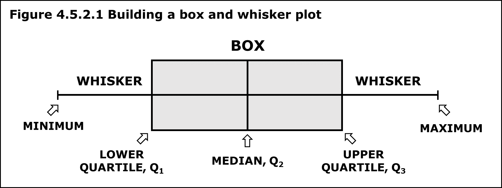
This diagram shows how a boxplot represents the minimum, lower quartile, median, upper quartile, and maximum on a number line, highlighting the IQR and overall range. Source.
The median, quartiles, and extremes organize the plot’s structure, and their positions relative to one another reveal important insights about the dataset. Because these elements summarize large amounts of information, they allow comparisons and interpretations that remain grounded in statistical reasoning.
Distribution symmetry, skewness, and variability can be identified from the spacing and relative lengths found in graphical summaries. These visual cues support context-driven claims, helping analysts understand whether the data cluster centrally, spread widely, or exhibit patterns that might warrant further investigation.
Skewness: The degree to which a distribution is pulled toward one side, indicated visually by longer whiskers or uneven spacing around the median in graphical summaries.
Interpreting skewness correctly matters because it influences how measures of center relate to each other. Recognizing this relationship is central to understanding what the data show and how to describe them accurately.
Interpreting the Mean–Median Relationship in Graphical Context
Although the mean is not shown directly in a boxplot, its inferred position relative to the median can be described based on the distribution’s shape. When a distribution is symmetric, the mean and median are typically close together. When it is right-skewed, the mean tends to lie to the right of the median; when left-skewed, it usually lies to the left.
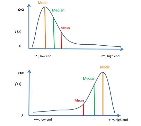
This figure illustrates how the mean shifts toward the longer tail in skewed distributions, while the median remains more central; the mode is included as an extra detail beyond the syllabus. Source.
These interpretations strengthen claims by connecting visual impressions to underlying numerical relationships.
Because boxplots rely on quartiles rather than raw data values, they highlight positional differences in spread more clearly than other graphs. This makes them powerful tools for discussing how the median divides the dataset and how unequal distances between quartiles or whiskers illustrate skewness.
Using Graphically Displayed Summary Statistics to Make Claims
When summary statistics appear in a graphical form, they support claims through clarity and structure. Students should pay particular attention to the following elements when making statements about data:
Median location
Indicates the central point of the distribution.
Its relative position inside the box can hint at symmetry or skewness.
Box width (IQR)
Shows the spread of the middle 50 percent of values.
Wider boxes correspond to more variability within that central range.
Whisker lengths
Reveal potential skewness: a longer whisker suggests a stretched tail.
Help identify the range of non-outlier observations.
Potential outliers
Displayed as separate points and indicate unusual observations that may influence interpretation.
These features must be interpreted together rather than in isolation. Students should refer consistently to the context of the data, using the visual characteristics to justify statements about trends, comparisons, or unusual behaviors present in the dataset.
Connecting Graphical Features to Distribution Characteristics
Graphical summaries reveal whether a distribution is symmetrical, right-skewed, or left-skewed, and each shape carries interpretive implications. Symmetrical distributions suggest balanced variability on both sides of the median. Right-skewed distributions display a concentration of lower values with a longer tail on the higher end, while left-skewed distributions show the opposite pattern. Students must recognize that these visual differences influence how summary statistics, such as the mean and median, relate.
Symmetry: A property of a distribution in which the left and right sides of a graph mirror each other around the center point.
These relationships support informed conclusions about the data. For instance, understanding from a boxplot that a dataset exhibits right skewness would justify a claim that the mean exceeds the median, even without calculating either value.
Applying Graphical Interpretation to Support Contextual Reasoning
Interpreting summary statistics graphically involves both identifying features and explaining their meaning in context. Students must articulate not only what the graph shows but also why those features matter. For example, noting that a distribution has a wide IQR should lead to a claim about substantial variability within the central 50 percent of observations. Observing a cluster of outliers supports statements regarding unusual behavior within the dataset.
By integrating visual evidence with clear reasoning about summary statistics, students enhance their ability to draw accurate, contextually grounded conclusions about quantitative data.
FAQ
Small differences in spacing can indicate subtle shape characteristics, even when the overall distribution appears roughly symmetric.
If the distance from Q1 to the median is only slightly larger or smaller than the distance from the median to Q3, this may suggest weak skewness that would not appear obvious from whisker length alone.
Slight asymmetry in quartile spacing may also indicate clustering within part of the central 50 percent, helping analysts refine claims about where values tend to concentrate.
It becomes misleading when sample sizes are small because sampling variability can distort quartile positions, making skewness harder to judge reliably.
It is also risky when the distribution contains multiple clusters. A boxplot only displays quartiles, so it cannot reveal multimodality and may suggest symmetry even when the raw data are unevenly structured.
If outliers pull the box or whiskers disproportionately, the inferred position of the mean may be inaccurate, even if the median–quartile spacing appears balanced.
Boxplots display only five statistics, so many different shapes can produce identical quartile and extreme values.
Two datasets may differ because:
• One may be unimodal while the other is bimodal.
• One may include subtle internal clustering hidden within quartile boundaries.
• The tails may differ in density even if the whisker endpoints match.
Thus, boxplots are effective for comparing locations and spreads but cannot reveal all distributional features.
Outliers should be assessed not only as statistical anomalies but in terms of whether they represent meaningful deviations in the real-world situation.
Consider whether:
• The value could result from measurement error.
• The context makes extreme values plausible.
• The outlier’s presence affects the interpretation of variability or performance.
Where context supports the value’s validity, the outlier may provide important insights rather than being dismissed as an artefact.
Skewness typically appears as systematic imbalance in whisker length or quartile spacing, whereas isolated outliers appear as individual points detached from the whiskers.
A distribution is more likely skewed if:
• One whisker is noticeably longer than the other.
• Quartile spacing is uneven across the median.
If the whiskers are balanced but one extreme point lies beyond the whisker tip, the shape is likely symmetric with an isolated anomaly rather than genuinely skewed.
Practice Questions
Question 1 (1–3 marks)
A boxplot summarises the distribution of the number of hours students studied for an examination. The median is positioned closer to the upper quartile than to the lower quartile, and the lower whisker is noticeably longer than the upper whisker.
(a) What does this suggest about the skewness of the distribution?
(b) Explain briefly how the position of the median supports your conclusion.
Question 1
(a)
• 1 mark: Identifies the distribution as left-skewed (negatively skewed).
(b)
• 1 mark: Explains that the median being closer to the upper quartile indicates more values clustered at the higher end.
• 1 mark: States that the longer lower whisker suggests a longer tail of lower values, supporting left skewness.
Total: 2–3 marks depending on clarity and correctness.
Question 2 (4–6 marks)
A company compares delivery times (in minutes) for two warehouses, A and B, using side-by-side boxplots. The boxplot for Warehouse A shows a larger interquartile range, a median slightly left of centre within the box, and two high-value outliers. Warehouse B has a narrow box, whiskers of similar length, and no outliers.
(a) Describe fully the shape, centre, and spread of the distribution for Warehouse A.
(b) Compare Warehouse A and Warehouse B in terms of centre and variability.
(c) Using the graphical information, suggest which warehouse demonstrates more consistent delivery performance and justify your answer.
Question 2
(a)
• 1 mark: Notes that the median being left of centre suggests slight right skewness.
• 1 mark: Describes the large interquartile range, indicating substantial variability.
• 1 mark: Mentions presence of high-value outliers indicating unusually long delivery times.
(b)
• 1 mark: Correctly compares medians, noting which warehouse appears to have shorter or longer typical delivery times based on median position.
• 1 mark: States that Warehouse A shows greater variability (larger IQR and outliers) while Warehouse B is more tightly clustered (smaller IQR).
(c)
• 1 mark: Identifies Warehouse B as more consistent.
• 1 mark: Provides justification using graphical evidence such as similar whisker lengths, smaller IQR, and absence of outliers.
Total: 5–6 marks depending on detail and accuracy.
