Understanding marginal and conditional relative frequencies is essential for analyzing two categorical variables, revealing patterns and associations by comparing proportions rather than raw counts within a two-way table.

Calculating Marginal and Conditional Relative Frequencies

Marginal and conditional relative frequencies provide structured ways to examine relationships between two categorical variables, helping to determine whether the variables may be associated. These measures rely on proportions rather than raw values, making them central to interpreting two-way (contingency) tables in a meaningful statistical context.

Two-Way Tables and Observed Frequencies

A two-way table organizes data for two categorical variables by listing the categories of one variable in the rows and the categories of the second variable in the columns. Each cell in the table displays the frequency (count) of observations that fall into the corresponding row–column combination.

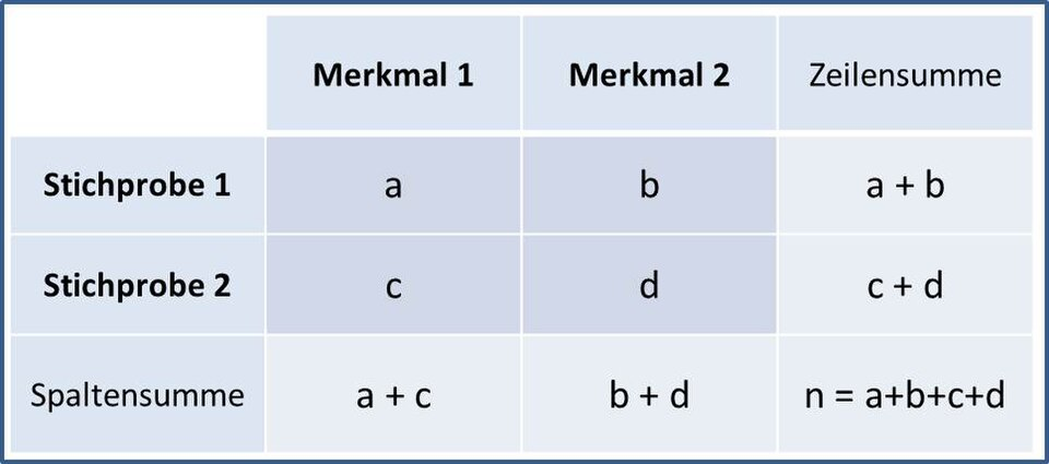
A 2×2 contingency table showing cell counts and marginal totals, illustrating the foundational structure used to compute joint, marginal, and conditional frequencies. German labels and references to the chi-square fourfold test appear but extend beyond the syllabus requirements while not affecting the table’s conceptual clarity. Source.

The totals along the margins are essential for computing relative frequencies.

A two-way table contains three types of totals that play distinct roles: row totals, column totals, and the grand total. These allow for calculating proportions that describe how the data are distributed within and across variable categories.

Marginal Relative Frequencies

Marginal relative frequencies describe the proportion of the total number of observations that fall into each row category or each column category. They highlight how frequently each category appears in the overall dataset, regardless of the category of the other variable.

Marginal relative frequencies provide an overall view of each variable’s distribution, helping students compare category sizes and understand baseline proportions.

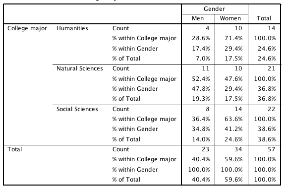
A contingency table displaying gender by major with percentages in each cell, illustrating how marginal totals and conditional distributions can be read directly from a two-way table. The specific majors and exact percentages extend slightly beyond the syllabus but faithfully represent the structural features needed for interpreting relative frequencies. Source.

Because they use the total number of observations as the denominator, they reflect broad patterns rather than conditional ones.

Conditional Relative Frequencies

Conditional relative frequencies offer more specific insight. A conditional relative frequency describes the proportion of observations that fall into a particular cell category, given that the observation belongs to a specific row or column. In other words, it restricts the comparison to a subset determined by one variable.

These relative frequencies make it possible to analyze how the distribution of one variable differs across categories of the second variable. Conditional frequencies are essential for identifying potential associations, because differences in conditional distributions across categories may suggest that the variables are related.

How to Compute Marginal and Conditional Relative Frequencies

Organizing clean, clearly labeled two-way tables ensures that marginal and conditional relative frequencies can be calculated accurately and interpreted confidently. Students should follow a systematic approach when working with two-way categorical data.

Process for Marginal Relative Frequencies

• Identify the row total or column total associated with the category of interest.

• Locate the grand total, which is the sum of all cell frequencies in the table.

• Compute the proportion using the formula:

  • Row marginal proportion = (row total) ÷ (grand total)

  • Column marginal proportion = (column total) ÷ (grand total)

• Interpret the resulting proportion in the context of the variable alone.

Process for Conditional Relative Frequencies

• Choose whether the condition is based on a row or a column.

• Identify the total for that row or column.

• Divide the relevant cell frequency by this row or column total.

• Interpret the resulting proportion as describing the distribution of one variable within the category of the other variable.

Because conditional relative frequencies rely on a restricted total, they reveal within-group patterns that marginal relative frequencies cannot capture.

Interpreting Marginal and Conditional Relative Frequencies

Interpreting relative frequencies requires comparing proportions and considering how distributions differ across conditions. Marginal relative frequencies show overall category prevalence, while conditional relative frequencies reveal meaningful variation between subgroups.

Using Marginal Relative Frequencies for Insights

• They allow comparisons of category sizes across the entire dataset.

• They are necessary for establishing broad context before looking at associations.

• They help identify imbalances or dominant categories in the data.

Using Conditional Relative Frequencies to Identify Associations

• Differences across conditional distributions often suggest that variables may be associated.

• Similar conditional distributions across categories typically suggest no association.

• They provide the foundation for deeper statistical investigations, including later inference procedures.

By analyzing conditional relative frequencies, students gain insight into whether patterns observed in data are consistent with meaningful relationships or may simply reflect random variation.