
AP Syllabus focus:
‘Explores how to interpret the correlation coefficient within the context of linear relationships (DAT-1.C). It explains that r is unit-free and elaborates on the significance of its value range from -1 to 1. A special emphasis on the meaning of r=0, r=1, and r=-1, illustrating perfect, no, and inverse linear relationships, respectively. Additionally, it addresses the critical point that correlation does not imply causation, explaining that a relationship between two variables does not mean one causes the other to change.’
The correlation coefficient is a central tool for understanding linear relationships in bivariate quantitative data. These notes explain how to interpret its value and meaning within statistical contexts.
Interpreting the Correlation Coefficient
The correlation coefficient, denoted r, provides a numerical measure of the direction and strength of a linear relationship between two quantitative variables. Because correlation plays a key role in judging how closely data points follow a straight-line pattern, it is essential to understand both what r can tell us and what it cannot.
The Unit-Free Nature of r
One of the most important characteristics of the correlation coefficient is that it is unit-free. This means its value does not depend on the units of measurement for either variable. Whether a dataset is measured in inches or centimeters, dollars or euros, seconds or minutes, the correlation coefficient remains unchanged. The absence of units makes r particularly useful for comparing relationships across different contexts and variable types.
Correlation Coefficient (r): A numerical measure, ranging from –1 to 1, that describes the direction and strength of the linear association between two quantitative variables.
Because r is standardized, its value communicates the same type of information regardless of scale or variable magnitude.
The Range of the Correlation Coefficient
The value of r always falls between –1 and 1, inclusive. This restricted range ensures that the interpretation of correlation is consistent across different situations.
Key meanings of extreme and central values include:
r = 1: A perfect positive linear relationship; all data points lie exactly on a line with positive slope.
r = –1: A perfect negative linear relationship; all data points lie exactly on a line with negative slope.
r = 0: No linear relationship; knowing the value of one variable does not help predict the other in a linear manner.
The closer r is to either extreme, the more strongly the data follow a linear pattern. Values near zero indicate weak or nonexistent linear association.
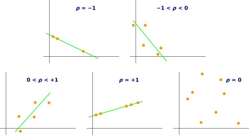
Scatterplots illustrating how different values of the correlation coefficient reflect changes in direction and strength of association. Tighter clustering around a straight line indicates stronger linear relationships. The notation uses ρ, the population correlation coefficient, which conveys the same conceptual meaning as the sample correlation r. Source.
Direction of the Linear Relationship
The sign of r communicates direction:
Positive r: As x increases, y tends to increase.
Negative r: As x increases, y tends to decrease.
The direction is one of the simplest and most informative features of correlation, helping to classify relationships quickly and precisely.
Strength of the Linear Relationship
The absolute value of r determines the strength of the linear association. Larger magnitudes correspond to stronger linear patterns. While AP Statistics does not require strict numerical cutoffs, general guidance includes:
|r| close to 1: Strong linear association
|r| around 0.5: Moderate linear association
|r| near 0: Weak or no linear association
Strength refers specifically to linearity; a strong nonlinear pattern may still have a correlation near zero.
Correlation and Linearity
Because correlation describes linear association, it may not reflect more complex patterns. Data forming curved or clustered relationships may have misleadingly low or moderate correlation values. Visual inspection using scatterplots remains a crucial tool for confirming that a linear model is appropriate before relying on r for interpretation.
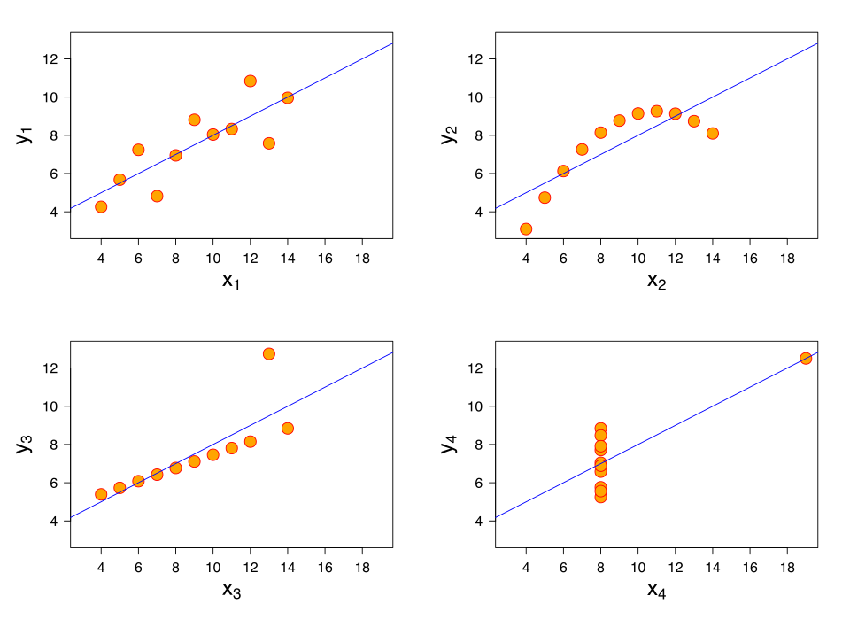
Anscombe’s quartet demonstrates that datasets with identical correlation values can possess dramatically different shapes and behaviors, emphasizing the importance of confirming linearity visually. Despite sharing the same correlation and regression line, each panel exhibits a distinct underlying pattern. Additional statistical similarities across the four datasets exceed syllabus requirements but reinforce the need to interpret r in context. Source.
Important Caveat: Correlation Does Not Imply Causation
A critical principle emphasized in this subsubtopic is that correlation does not imply causation. Even if two variables exhibit a strong linear association, this does not mean one variable causes changes in the other. Several factors can produce correlations without causation:
Confounding variables that influence both x and y
Common underlying causes
Coincidence or randomness, especially in small samples
Reverse causation, where the direction of influence is opposite what might be assumed
Understanding this limitation is essential for correctly interpreting r in real-world contexts. Many misinterpretations in media and public discussions arise from confusing correlation with evidence of causal impact.
Interpreting Correlation in Context
Effective interpretation always requires attention to the specific variables being studied. When analyzing a correlation:
Consider whether the relationship is appropriate to model linearly.
Assess the direction and strength within the context of the data.
Evaluate whether the correlation makes logical sense based on subject knowledge.
Remember that correlation alone cannot justify claims of causation.
These elements ensure that r contributes meaningfully to the broader analysis of bivariate quantitative data.
Summary of Key Interpretive Points
r is unit-free, enabling comparison across data types.
The value always lies between –1 and 1.
Sign indicates direction; magnitude indicates strength.
r measures linear, not general, association.
Correlation does not imply causation under any circumstances.
These characteristics allow the correlation coefficient to serve as a foundational measure in AP Statistics, guiding interpretations of how two quantitative variables relate within a linear framework.
FAQ
The correlation coefficient is calculated using standardised values of the variables, which ensures the measure cannot exceed the limits of a perfect linear fit.
These bounds reflect the mathematical structure of covariance relative to the standard deviations of the variables. A value of 1 or –1 occurs only when all points lie exactly on a straight line, making any larger value impossible.
Because r is confined to this interval, it provides a consistent scale for interpreting the strength of linear association.
Yes. Correlation only measures linear association, so any curved or cyclical pattern may produce an r value close to zero even when the relationship is strong.
Examples include quadratic patterns, U-shaped associations, and sinusoidal patterns. These relationships can be highly predictable but still yield a low correlation because the data do not cluster around a straight line.
Outliers can dramatically increase or decrease the value of r because they affect both the covariance and the spread of the data.
An extreme point may artificially strengthen or weaken the correlation, giving a misleading view of the overall pattern.
To evaluate the impact of outliers, it is useful to check:
• scatterplots before interpreting r
• correlation with and without the outlier
• whether the outlier reflects an error or a valid data value
Yes. Correlation summarises only direction and strength, not the form or context of the data.
Two datasets may:
• have identical r values but different spreads
• include different numbers of outliers
• show distinct underlying mechanisms
This is why visual inspection is essential, as datasets with the same numerical r can behave very differently.
In small samples, correlation values can vary widely due to random fluctuation, making strong or weak values less reliable.
Larger samples stabilise the estimate of r, making it a more trustworthy indicator of the true relationship.
When interpreting r:
• be cautious with small samples
• consider whether the sample size is large enough to reflect a consistent pattern
• rely on graphical analysis alongside correlation for context
Practice Questions
Question 1 (1–3 marks)
A study finds that the correlation between students’ weekly hours of study and their exam score is r = 0.78.
Explain what this value of r indicates about the relationship between the two variables.
State one thing this value of r does not imply.
Question 1 (3 marks total)
• 1 mark: States that r = 0.78 indicates a positive relationship, such that students who study more tend to have higher exam scores.
• 1 mark: States that the association is fairly strong or moderately strong.
• 1 mark: Clearly states that correlation does not imply causation, or gives an equivalent statement (e.g., r does not prove that studying more causes higher scores).
Question 2 (4–6 marks)
A researcher records data on the number of hours people spend exercising each week and their resting heart rate. The correlation between the two variables is r = –0.62.
(a) Interpret the direction and strength of this correlation.
(b) Explain why a correlation of this magnitude does not guarantee that a straight-line model is appropriate for the data.
(c) The researcher concludes that increasing exercise causes a reduction in resting heart rate. Explain why this conclusion may not be justified based on correlation alone.
Question 2 (6 marks total)
(a) 2 marks:
• 1 mark: Identifies the relationship as negative (as exercise increases, resting heart rate tends to decrease).
• 1 mark: Identifies that the association is moderate or moderately strong.
(b) 2 marks:
• 1 mark: States that correlation only measures linear association.
• 1 mark: States that the data may not follow a straight-line pattern or could show curvature or unusual points.
(c) 2 marks:
• 1 mark: States that correlation alone cannot establish causation.
• 1 mark: Gives a reason such as confounding variables, possible reverse causation, or another factor influencing both exercise and heart rate.
