
AP Syllabus focus:
‘This section will introduce the concept of simple linear regression models, explaining how they use an explanatory variable (x) to predict a response variable (y). It will detail the basic idea behind regression, its purposes, and how it fits into the broader context of bivariate data analysis.’
Linear regression provides a foundational statistical method for examining how one quantitative variable can be used to predict another, helping uncover structured relationships within bivariate data.
Understanding the Purpose of Linear Regression
Linear regression offers a systematic way to study the relationship between two quantitative variables by modeling how changes in one variable are associated with changes in another. In AP Statistics, the focus is on simple linear regression, which involves one explanatory variable and one response variable. The explanatory variable is the variable whose values are used to account for, explain, or predict the values of the response variable. The response variable is the outcome or measurement being predicted or described. This framework allows students to move beyond describing relationships to creating predictive models grounded in statistical reasoning.
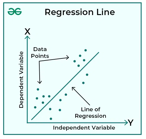
Scatterplot with a regression line showing how a straight-line model summarizes the relationship between an explanatory variable xxx and a response variable yyy. The points represent observed data, while the line shows the model’s predicted response for each value of xxx. This image focuses only on the essential features needed at this stage: axes, data points, and the line of best fit. Source.
The Role of Bivariate Quantitative Data
Simple linear regression is applied only to bivariate quantitative data, meaning data that include numerical measurements of two variables for each individual in a sample or population. Before building a regression model, variables must be confirmed as quantitative because regression techniques rely on numerical relationships. Bivariate quantitative data make it possible to represent relationships visually with scatterplots and analytically through model-building. The regression model formalizes what patterns in the data suggest by estimating a mathematical rule linking the two variables.
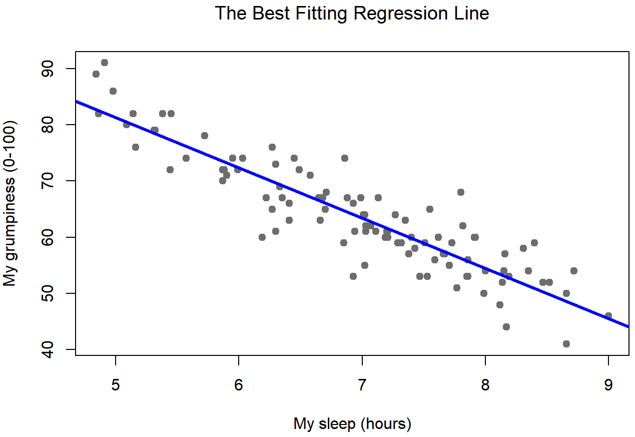
Scatterplot of grumpiness as a function of hours slept, with the best-fitting regression line drawn through the cloud of points. The line passes roughly through the middle of the data, illustrating how a regression model summarizes the overall linear trend while individual points still show variation. The specific sleep–grumpiness context is extra detail beyond the AP syllabus, but it serves as a concrete example of using one quantitative variable to predict another. Source.
Foundations of Linear Regression Models
A linear regression model aims to capture a straight-line relationship between an explanatory variable and a response variable. This relationship is represented through a regression equation, which provides predicted values of the response variable based on input values of the explanatory variable. The central idea is that while individual data points may vary, their overall pattern can often be approximated with a line that summarizes the trend.
Linear Regression Model: A statistical model that uses a straight-line equation to describe how a response variable is predicted from an explanatory variable.
A regression model suggests how one might expect the response variable to change when the explanatory variable increases or decreases. When interpreting this model, it is essential to recognize that regression does not establish causation but instead quantifies association and predictive strength within the observed data context.
The Regression Equation
In simple linear regression, predictions are generated using a linear equation that reflects the relationship between variables. The equation uses two components: a slope, representing the predicted rate of change in the response variable, and a y-intercept, representing the predicted response value when the explanatory variable equals zero.
EQUATION
= Predicted value of the response variable
= y-intercept of the regression line
= slope of the regression line
= value of the explanatory variable
The regression equation forms the backbone of prediction in AP Statistics.
Interpreting the Components of the Model
Each part of the regression equation carries meaningful statistical interpretation. The slope indicates how much the predicted response variable changes, on average, for each one-unit increase in the explanatory variable. A positive slope suggests an increasing relationship, whereas a negative slope reflects a decreasing association. The y-intercept, while sometimes lacking practical meaning depending on the context, represents the predicted response when the explanatory variable is zero. In many real-world situations, such a value may fall outside the range of observed data, so its interpretability must always be evaluated within the study’s context.
Why Linear Regression Matters in Data Analysis
Linear regression models serve several important purposes in statistical investigations. They provide structure to relationships that appear linear in scatterplots, create a systematic tool for prediction, and supply quantitative measures that assess how well the model fits the data. By summarizing an entire set of bivariate observations with a single linear rule, regression allows researchers and students to evaluate trends, compare predicted and observed values, and examine how strongly variables are associated. This process ties directly to the broader goals of two-variable data analysis, where identifying and modeling relationships plays a central role in statistical reasoning.
How Linear Regression Fits into the Broader Analytical Framework
The introduction to linear regression situates students at the beginning of a sequence of analytical tools used for deeper exploration of relationships between variables. Understanding the regression model prepares learners for later topics such as interpreting slopes and intercepts, analyzing residuals, and evaluating model appropriateness. By establishing how predictions emerge from a linear structure, this subsubtopic builds essential skills for assessing the quality and limitations of statistical models. In AP Statistics, linear regression marks the transition from descriptive study of patterns to predictive and inferential thinking about real-world data.
FAQ
A regression line is calculated using a precise statistical procedure that minimises the total squared vertical distances between data points and the fitted line. This ensures an objective and reproducible result.
A line drawn by eye depends on judgement and may vary between individuals, potentially missing the true underlying pattern in the data. Regression provides a mathematically optimal line, not a subjective approximation.
Linear regression relies on numerical relationships so that changes in one variable can be expressed as mathematical increases or decreases in the other.
Categorical variables cannot form meaningful numerical scales for predicting a value, so the model would fail to represent the relationship appropriately.
Yes. A clearer, more tightly clustered linear pattern generally yields more consistent predictions.
When the points are widely scattered, the linear trend may be weak. In such cases, predictions from the regression model may vary greatly because the line does not closely represent the data.
The y-intercept reflects the predicted value of the response when the explanatory variable is zero, but this scenario may not always be realistic.
For example, zero units of the explanatory variable might fall outside the plausible or observed range. In such cases, the intercept is simply a mathematical result, not a meaningful contextual prediction.
Evidence against linearity may include:
• Curved patterns
• Clusters of points indicating multiple groups
• Clear changes in trend at different values of the explanatory variable
When these features appear, a straight-line model may misrepresent the relationship, reducing interpretive accuracy.
Practice Questions
Question 1 (1–3 marks)
A researcher records the number of hours students revise (x) and their exam scores (y). She plans to use a simple linear regression model to predict exam score from hours revised.
(a) Identify the explanatory variable and the response variable in this context. (1 mark)
(b) Explain, in context, what the purpose of using a linear regression model would be for this data. (2 marks)
Question 1
(a)
• Explanatory variable: hours revised. (1 mark)
• Response variable: exam score. (1 mark if both correctly identified; 0 if reversed)
(b)
Award up to 2 marks:
• 1 mark for stating that the model is used to describe or summarise the relationship between hours revised and exam score.
• 1 mark for stating that the model can be used to predict exam scores based on the number of hours revised.
(Full 2 marks require both description and purpose in context.)
Question 2 (4–6 marks)
A scatterplot of two quantitative variables appears to show a roughly linear upward trend. A statistician decides to fit a simple linear regression model to predict Variable Y from Variable X.
(a) State one reason why a linear regression model might be appropriate based on the scatterplot. (1 mark)
(b) Explain the role of the slope and the intercept in a simple linear regression model. (2 marks)
(c) The statistician uses the model to predict Y for an X-value far outside the range of the data. Explain why this prediction may not be reliable. (2–3 marks)
Question 2
(a)
• 1 mark for noting that the scatterplot shows an approximately linear pattern or straight-line trend, suggesting linear regression is suitable.
(b)
Award up to 2 marks:
• 1 mark for describing the slope as representing the predicted change in Y for a one-unit increase in X.
• 1 mark for describing the intercept as the predicted value of Y when X is zero (even if its meaning may be limited in context).
(c)
Award up to 3 marks:
• 1 mark for identifying that predicting outside the observed range is extrapolation.
• 1 mark for stating that extrapolated predictions are unreliable because the model is based only on the observed data range.
• 1 mark for explaining that the true relationship may differ beyond the data used to create the model.
