
AP Syllabus focus:
‘Instructions on applying transformations to variables (e.g., taking the natural logarithm or squaring values) to achieve a more linear relationship for regression analysis. This includes creating transformed data sets, assessing the effectiveness of transformations through increased randomness in residual plots or movement of r² towards 1, and determining when the least-squares regression line of the transformed data provides a better model.’
Transforming data helps reveal linear patterns that are hidden in nonlinear relationships. These notes explain why transformations matter in regression and how students can apply them effectively.
Understanding Why Transformations Are Used
When analyzing nonlinear associations between two quantitative variables, a straight line may not describe the pattern well. In such cases, analysts apply transformations, which are mathematical re-expressions of the variables, to make the relationship more linear.
Transformation: A mathematical re-expression of a variable intended to straighten a curved pattern in bivariate data so that linear regression methods become more appropriate.
Transformations are valuable because many statistical tools, including least-squares regression, rely on the assumption of linearity. Transforming data can stabilize variability, clarify trends, and improve the interpretability of residual plots.
Common Types of Transformations
Although many transformations exist, the AP Statistics course emphasizes a few widely used ones. Each aims to straighten the form of the scatterplot or make the residual plot appear more random.
Logarithmic Transformations
A logarithmic transformation applies a natural log or base-10 log to one or both variables to linearize relationships that grow quickly but level off.
Natural Log Transformation: A re-expression in which the natural logarithm, , replaces the original value of a variable, often used to linearize exponential-type patterns.
A logarithmic transformation is particularly effective when the response variable increases at a decreasing rate or when ratios and proportional changes are relevant.
Power Transformations
Power transformations involve raising a variable to some exponent, such as squaring or taking the square root, to adjust curvature.
Power Transformation: A re-expression in which a variable is raised to a chosen power (e.g., or ) to reduce nonlinear patterns in data.
Power transformations can address situations where the rate of increase or decrease accelerates more dramatically than a logarithmic transformation can handle.
Creating Transformed Data Sets
To evaluate whether a transformation improves linearity, students construct a new data set using transformed values of the explanatory variable, the response variable, or both. The transformed data are then displayed in a revised scatterplot.
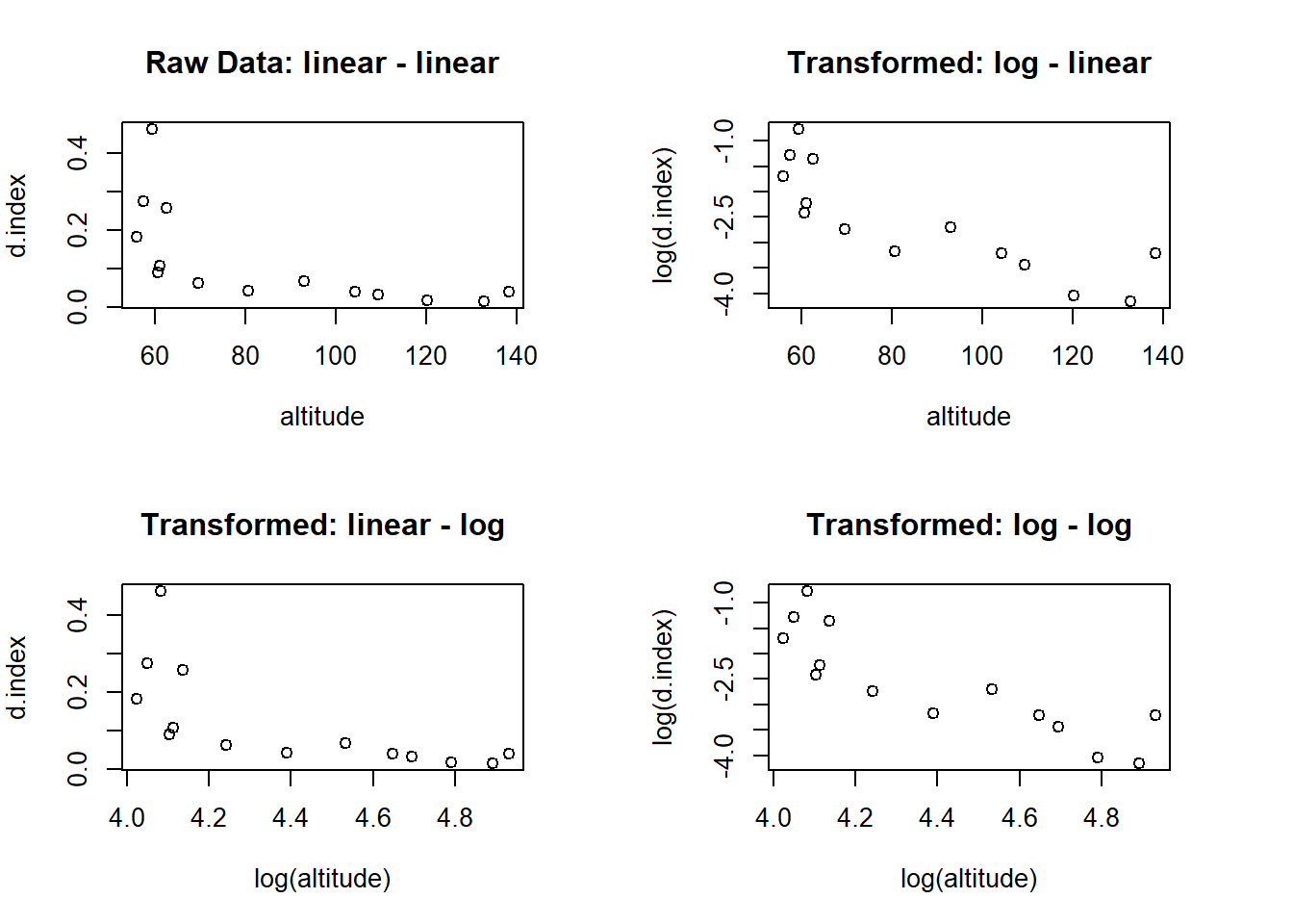
This panel of scatterplots compares untransformed data with three log-based transformations, illustrating how re-expression can straighten nonlinear patterns and improve linear model suitability. Source.
Key steps include:
Identifying whether the original scatterplot exhibits curvature.
Selecting an appropriate transformation based on the nature of the curvature.
Re-expressing the variable(s) to create transformed values.
Plotting the transformed data to inspect whether the relationship appears more linear.
Fitting a least-squares regression line to the transformed data.
These steps help ensure that the transformation meaningfully improves the model rather than distorting the relationship.
Assessing the Effectiveness of Transformations
A transformation is considered successful if it leads to a regression model that better meets the assumptions of linear regression.
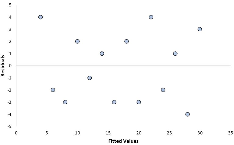
This residual plot demonstrates the random scatter expected when a linear model is appropriate, illustrating how a successful transformation produces no visible structure in the residuals. Source.
Indicators of improvement include:
Increased randomness of points in the residual plot.
Reduction in curved patterns, clusters, or funnel shapes in the residuals.
A movement of toward 1, signaling that a larger proportion of variation in the response variable is explained by the transformed model.
Residual Plot: A scatterplot of residuals versus explanatory variable values or predicted values used to assess whether a linear model is appropriate.
Residual plots are central to judging model quality, even after data are transformed.
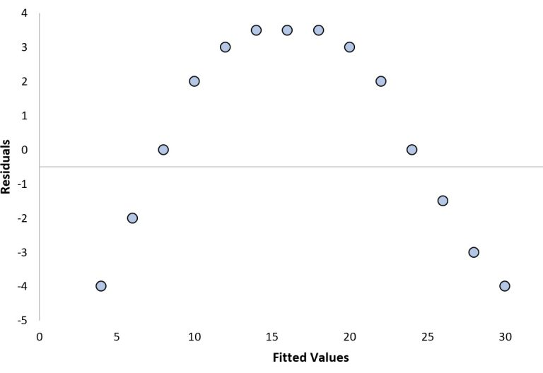
This residual plot displays a clear curved structure, indicating that the linear model is inadequate and that a transformation or different modeling approach is required. Source.
Interpreting Linear Regression After Transformation
When the transformed relationship appears more linear, students may fit a new least-squares regression line to the transformed data. The resulting regression coefficients describe how the transformed variables relate.
If the transformation meaningfully improves linearity, the new regression model will:
More accurately predict transformed response values.
Show a line that visually fits the transformed scatterplot more closely.
Produce residuals that show no systematic structure.
It is important to distinguish between interpreting the regression on the transformed scale and translating predictions back to the original units of measurement. Some transformations, such as logarithms, require exponentiating predicted values to return to original units.
Determining When a Transformed Model Is Better
Students should favor the transformed regression model when:
The transformed scatterplot shows a clearer linear pattern than the original.
The transformed residual plot indicates more randomness.
The transformed model has a substantially larger , reflecting stronger explanatory power.
These criteria ensure that the decision is based on statistical evidence rather than appearance alone. Transformations should always be guided by the goal of using linear regression responsibly and accurately.
FAQ
Different types of curvature hint at suitable transformations. If the plot shows rapid early growth that levels off, a logarithmic transformation of the response variable is often appropriate.
If the curvature accelerates as x increases, a power transformation such as squaring or square rooting may help.
Analysts typically inspect the direction and steepness of curvature before selecting a transformation, rather than choosing one randomly.
Yes. A transformation does not need to be applied to both variables.
Transforming only the explanatory variable can be helpful when curvature appears horizontally, while transforming only the response variable is useful when vertical curvature dominates.
The key principle is to adjust only the variable responsible for the nonlinear pattern rather than transforming both by default.
Transformations can reduce the influence of extreme values by compressing large numbers or expanding small ones.
However, a transformation does not remove outliers; it may simply lessen their impact on the fitted line.
After transforming data, analysts still need to verify whether any points remain unusually distant from the new pattern.
Both forms of logarithmic transformation have the same shape and will produce very similar scatterplots.
The decision is usually practical rather than mathematical: natural logs are more common in statistical software, while base-10 logs may be easier to interpret when values span several powers of ten.
Consistency within the analysis is more important than the specific base used.
When only the response variable is transformed, predictions must be reversed at the end of the analysis.
For example:
• If the response variable was log-transformed, predictions are converted back by exponentiating.
• If a square root transformation was used, predictions are squared to return to the original scale.
It is important to note that back-transformed predictions may not align perfectly with a model fitted on untransformed data due to the mathematical effects of transformation.
Practice Questions
Question 1 (1–3 marks)
A researcher analyses a nonlinear relationship between two quantitative variables and notices a curved pattern in the residual plot of the original regression model. The researcher applies a logarithmic transformation to the response variable.
Explain why this transformation might make a linear model more appropriate.
Question 1 (3 marks)
• 1 mark for stating that a logarithmic transformation can straighten a curved relationship.
• 1 mark for explaining that the transformation may stabilise variability or reduce curvature.
• 1 mark for explaining that a more linear pattern allows the assumptions of linear regression to be met (e.g., residuals become more random).
Question 2 (4–6 marks)
A data set shows a strongly curved relationship between variables x and y. A student applies a square root transformation to x and fits a new least-squares regression line.
After fitting the transformed model, the student observes the following:
• The scatterplot of the transformed data shows a clearer linear trend.
• The residual plot shows points randomly scattered around zero.
• The coefficient of determination increases from 0.62 to 0.84.
(a) Explain why a square root transformation may have been appropriate for this data set.
(b) Using the evidence provided, assess whether the transformed model is more suitable than the original model.
(c) State one reason why it is important to evaluate residual plots even after a transformation has been applied.
Question 2 (6 marks)
(a) (2 marks)
• 1 mark for stating that the square root transformation reduces curvature in data that increase or decrease rapidly.
• 1 mark for explaining that it can make the relationship closer to linear.
(b) (3 marks)
Award up to 3 marks:
• 1 mark for noting the more linear appearance of the transformed scatterplot.
• 1 mark for stating that the residual plot shows random scatter, indicating improved model fit.
• 1 mark for explaining that the increase in the coefficient of determination (0.62 to 0.84) provides strong evidence that the transformed model explains more variation.
(c) (1 mark)
• 1 mark for noting that residual plots help verify whether the linear model assumptions hold, even after transformation (e.g., checking for remaining patterns or non-constant variance).
