
AP Syllabus focus:
‘Detail the calculation of the mean (μx = np) and standard deviation (σx = sqrt(np(1-p))) for a binomial distribution, emphasizing these formulas' derivation and application. This subsubtopic explores the rationale behind these formulas and how they reflect the expected outcomes and variability of binomially distributed variables.’
Calculating Mean and Standard Deviation for a Binomial Distribution
This section develops the essential understanding that binomial distributions possess predictable numerical characteristics. These characteristics allow students to quantify expected outcomes and evaluate variability when studying repeated independent trials.
Understanding Parameters in Binomial Settings
A binomial distribution arises when a random variable counts the number of successes in a fixed number of independent trials, each with the same probability of success.
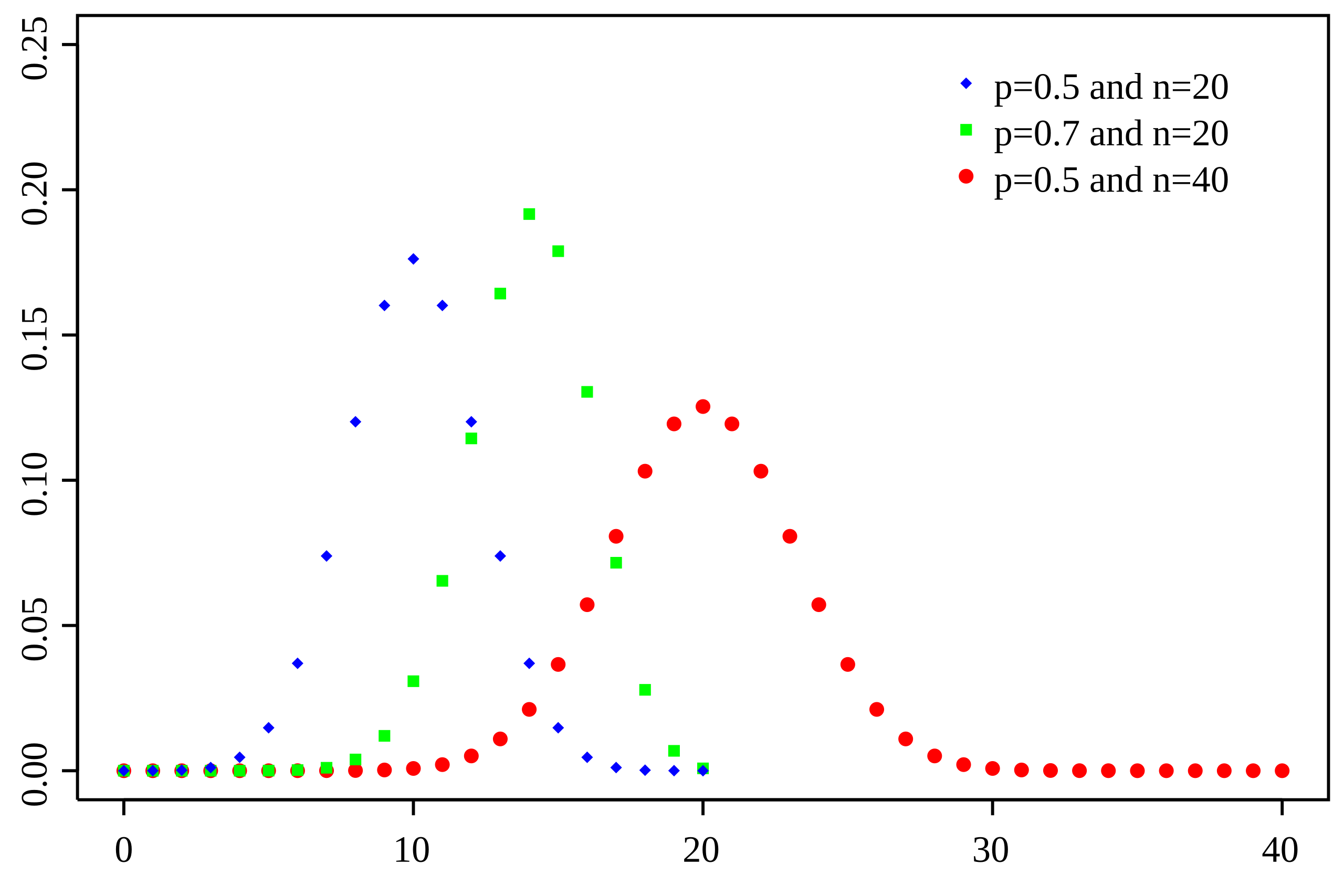
Binomial probability mass functions for several combinations of number of trials nnn and success probability ppp. Each dot represents the probability of obtaining a particular number of successes. The way the distributions shift and widen as nnn and ppp change illustrates how the mean npnpnp and standard deviation np(1−p)\sqrt{np(1-p)}np(1−p) govern the center and variability of a binomial distribution; the legend and multiple curves provide extra detail beyond what is strictly required by the syllabus. Source.
Within this structure, two key parameters describe the distribution’s behavior: the mean and the standard deviation. These parameters serve as numerical summaries of the typical long-run behavior of repeated binomial processes.
Before exploring how these parameters are calculated, it is important to recognize that each parameter provides different interpretive insight. The mean measures the distribution’s central tendency, while the standard deviation measures the typical size of deviations from the mean over many repetitions of the process.
Defining the Mean of a Binomial Distribution
The mean of a binomial distribution is also referred to as the expected value, a term that reflects what occurs on average across many iterations of the same random process.
Mean (Expected Value): The long-run average number of successes expected in repeated binomial trials.
In a binomial setting, the mean depends on two essential components: the number of trials and the probability of success. Understanding how these components combine mathematically helps clarify why the mean grows proportionally with both the number of opportunities for success and the likelihood of success in each trial.
EQUATION
= Number of independent trials
= Probability of success on each trial
The equation expresses the relationship between structural features of the binomial process and the resulting expected number of successes. It highlights that increasing the number of trials or increasing the chance of success systematically increases the long-run average of the distribution.
Understanding Variability in Binomial Outcomes
While the mean identifies the central expected result, the standard deviation provides a numerical description of how much variation exists around that mean.
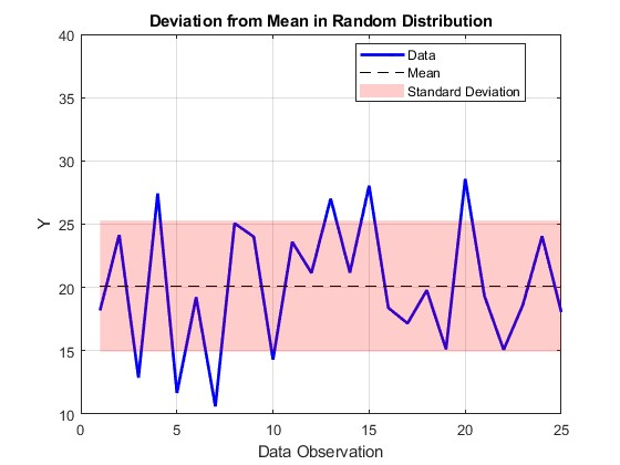
Line plot of sample data values with the mean marked by a dashed horizontal line and a shaded band representing one standard deviation above and below the mean. The vertical fluctuations of the data around the mean illustrate how standard deviation captures typical deviations from the center. The specific data set is arbitrary and not binomial, so it introduces extra contextual detail while still reinforcing the general concept of standard deviation used in this subsubtopic. Source.
Binomial outcomes vary because the number of successes achieved across repeated sets of trials is influenced by chance. A distribution with greater variability spreads its outcomes more widely, making the number of successes less predictable.
Standard Deviation: A numerical measure that describes the typical distance between the observed number of successes and the mean in a binomial distribution.
The standard deviation depends on both the probability of success and the probability of failure. This dependence reflects how the unpredictability of outcomes arises from the interaction between successes and failures within the same process.
EQUATION
= Number of independent trials
= Probability of success
= Probability of failure
Including both and in the formula highlights an important idea: variability is greatest when success and failure are equally likely, and it decreases when one outcome becomes more certain.
Interpreting the Role of Mean and Standard Deviation
Within the AP Statistics framework, these parameters are essential for describing and understanding the behavior of binomial random variables. Their interpretation supports deeper insight into repeated random processes by offering clear numerical benchmarks.
Key interpretive points include:
The mean tells how many successes students should expect in the long run when repeating the entire binomial process under identical conditions.
The standard deviation tells how much the actual number of successes typically varies from that expectation, offering a measure of predictability.
When the number of trials increases, the mean grows proportionally, while the standard deviation grows more slowly because of the square-root structure of the formula.
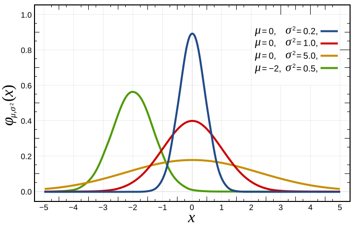
Probability density functions of several normal distributions with different means and variances. Curves with larger variance are wider and flatter, while curves with smaller variance are taller and more concentrated around their means, illustrating how standard deviation controls spread. This continuous example introduces extra detail beyond the binomial setting, but it reinforces the same relationship between parameters, center, and variability that underlies the binomial formulas for mean and standard deviation. Source.
When the probability of success approaches 0 or 1, the standard deviation shrinks, reflecting reduced uncertainty in outcomes.
Connecting Parameters to Real-World Reasoning
In applied statistical reasoning, parameters serve as essential tools because they summarize the behavior of random variables without requiring enumeration of every possible outcome. For a binomial distribution, the formulas for the mean and standard deviation provide compact and interpretable measures of expectation and variability.
Students should view these parameters not as abstract computations, but as meaningful descriptors that help quantify how random behavior unfolds across repeated trials. Their use supports reasoning about long-run patterns, comparisons between different binomial contexts, and communication of statistical insights using precise and appropriate units.
FAQ
The mean increases as the probability of success increases because the expected number of successes depends directly on that probability.
When p is small, the mean remains low even with many trials. As p approaches 1, the mean approaches the total number of trials, reflecting near-certain success on each trial.
Variability arises from the interaction between successes and failures. If either outcome becomes highly likely, the variability decreases because the results become more predictable.
The standard deviation reaches its maximum when p and 1 − p are close to 0.5, meaning both outcomes occur with similar likelihood.
Yes. Different combinations of n and p can result in the same value of n p (1 − p), which determines the standard deviation.
For example, increasing n while reducing p may produce a similar product, keeping the standard deviation unchanged.
A small standard deviation indicates that most outcomes cluster tightly around the mean.
This produces a distribution that is sharply peaked with little spread, reflecting predictable results and low random fluctuation.
For large n, small changes in p can significantly change both the mean and the standard deviation because each shift is scaled by the size of the trials.
Key effects include:
• A slight increase in p noticeably increases the mean.
• The standard deviation may grow or shrink depending on whether the change in p moves the distribution towards or away from its maximum variability point near p = 0.5.
Practice Questions
Question 1 (1–3 marks)
A factory produces light bulbs, and each bulb has a 0.04 probability of being defective. A quality inspector randomly selects 50 bulbs.
Assuming the number of defective bulbs follows a binomial distribution, calculate the mean and the standard deviation of the number of defective bulbs in the sample.
Question 1 (1–3 marks)
• 1 mark: Correct identification of mean = np.
• 1 mark: Correct calculation of mean = 50 × 0.04 = 2.
• 1 mark: Correct calculation of standard deviation = sqrt(50 × 0.04 × 0.96) = sqrt(1.92) ≈ 1.385.
Total: 3 marks.
Question 2 (4–6 marks)
A charity receives donations from individuals during an online campaign. Each visitor to the donation page independently decides whether to donate, with a constant probability of 0.12.
Let X represent the number of visitors who donate out of the next 200 visitors.
(a) Explain why X can be modelled using a binomial distribution.
(b) Calculate the expected number of donations.
(c) Calculate the standard deviation of X.
(d) Interpret the standard deviation in context.
Question 2 (4–6 marks)
(a) (2 marks)
• 1 mark: States that each trial (visitor) has two outcomes: donate or not donate.
• 1 mark: States that trials are independent with constant probability of success (0.12), and there is a fixed number of trials (200).
(b) (1 mark)
• Correct calculation of mean = np = 200 × 0.12 = 24.
(c) (2 marks)
• 1 mark: Correct use of formula standard deviation = sqrt(np(1 − p)).
• 1 mark: Correct calculation = sqrt(200 × 0.12 × 0.88) = sqrt(21.12) ≈ 4.595.
(d) (1 mark)
• Provides a correct contextual interpretation, e.g.:
“On average, the number of donors typically varies by about 4 to 5 from the expected value of 24.”
Total: 6 marks.
