
AP Syllabus focus:
‘Learning Objective UNC-3.D & UNC-3.D.1: Focus on the interpretation of probabilities and parameters (mean and standard deviation) of a binomial distribution, including how to contextualize these statistical measures within specific scenarios or populations. This involves understanding the significance of these parameters in real-world contexts and using appropriate units for interpretation.’
Interpreting parameters of a binomial distribution helps students understand how probability models translate into meaningful, context-specific insights about expected outcomes and their variability across repeated, identical trials.
Understanding the Role of Parameters in Interpretation
Interpreting binomial distribution parameters requires understanding how the mean and standard deviation describe long-run behavior of a binomial random variable within a meaningful real-world context. These parameters make probability statements actionable by linking the theoretical model to the scenario being investigated.
The Meaning of the Mean in Context
The mean of a binomial random variable represents the long-run average number of successes across many repetitions of a binomial process. When interpreting this value, attention must be paid to the population, measurement units, and the assumptions of the binomial setting, such as fixed number of trials, constant probability of success, and independence.
Mean (Expected Value): The long-run average number of successes predicted by a binomial probability model for a specified number of identical trials.
When applying the mean to a real situation, it is essential to state what constitutes a “success,” how many trials are involved, and the population or scenario reflected by the distribution. The clarity of this contextual interpretation allows readers or decision makers to understand the expected outcome in practical terms rather than as an abstract numerical value.
EQUATION
= Total number of binomial trials
= Probability of success on each trial
The mean provides a reference point for anticipating typical performance, but it does not imply that the observed number of successes in any single trial sequence will equal this value. Graphically, the binomial distribution’s shape, center, and spread provide intuition for these parameters: the mean marks the distribution’s balance point and the standard deviation reflects how concentrated or diffuse the bars are around that center.
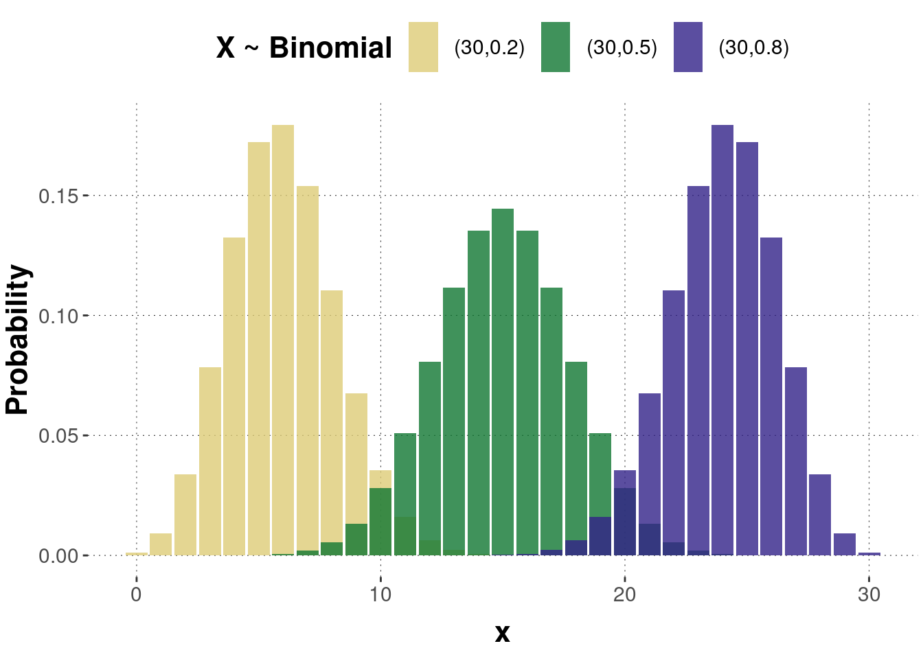
The figure compares three binomial distributions with identical numbers of trials but different probabilities of success, illustrating how the mean shifts and the spread changes with ppp. Students should notice how parameter pairs (n,p)(n,p)(n,p) control the center and concentration of probability mass. Source.
Understanding Standard Deviation as a Measure of Variability
The standard deviation of a binomial distribution measures the typical distance between the actual number of successes and the mean number of successes across repeated trials. Interpreting this value requires attention to units, just as with the mean, because the standard deviation describes variability in the same units as the number of successes.
Standard Deviation: A measure describing the typical amount by which the number of observed successes differs from the mean number of successes in a binomial distribution.
This measure is crucial for evaluating the stability or uncertainty associated with the process. A larger standard deviation indicates greater variability, meaning outcomes may fluctuate widely from trial to trial. A smaller standard deviation suggests more consistent results, clustered closer to the mean.
EQUATION
= Total number of binomial trials
= Probability of success
= Probability of failure
The standard deviation plays a central role in contextual conclusions by describing how predictable the binomial process is and how much variation should be anticipated in real applications. Interpreting the parameters involves more than quoting their numerical values; it means using them to decide which ranges of counts are typical and which are rare in the long run.
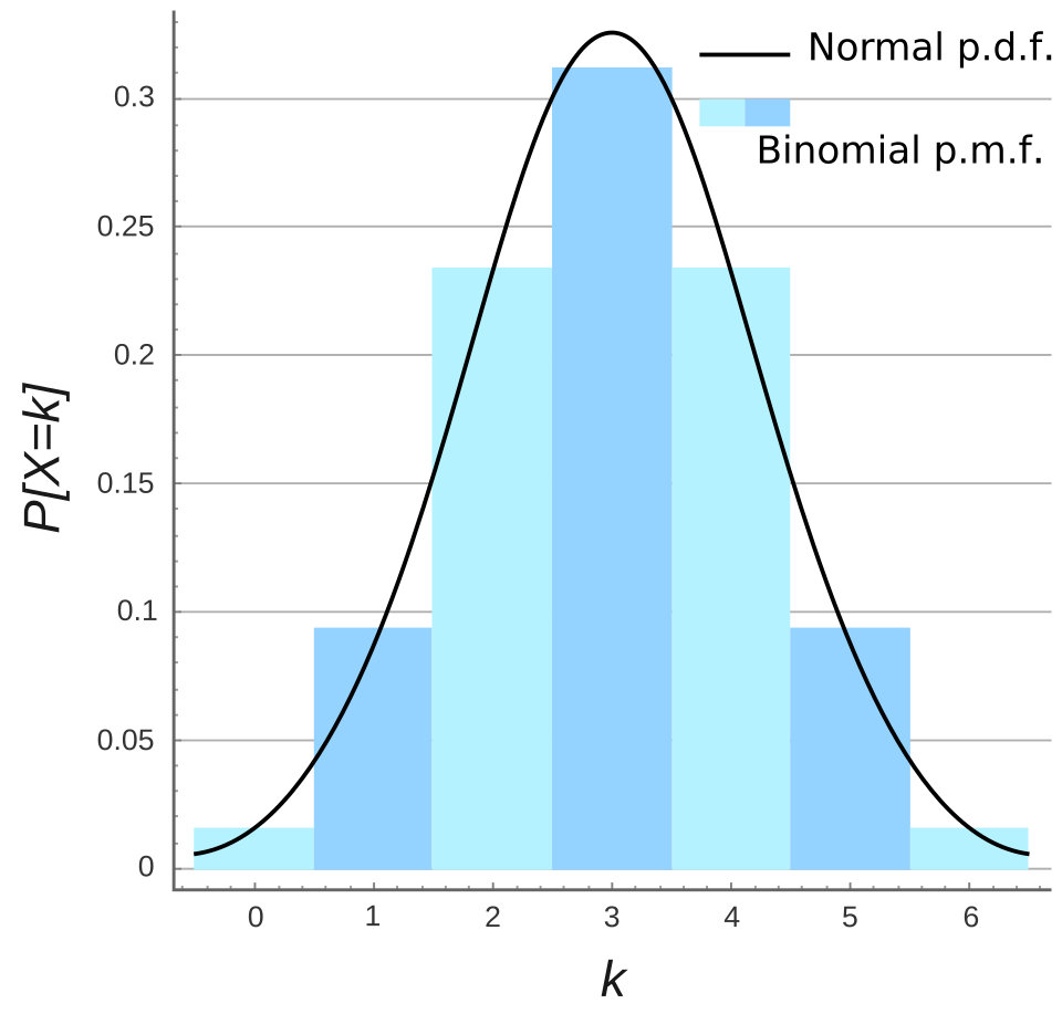
The bars represent the binomial distribution’s probabilities, with the highest bars near the mean and the lowest in the tails. The overlaid normal curve is additional context not required here; students should focus on how the bar heights show typical and rare counts of successes. Source.
Interpreting Probabilities in Relation to Parameters
In a binomial model, probabilities describe the likelihood of observing certain numbers of successes. When interpreting these probabilities, students should relate them to both the mean and the spread of the distribution. This connection helps explain whether a given outcome is typical or unusual for the modeled scenario.
Key interpretive points include:
Linking the probability of observing a number of successes to its distance from the mean.
Assessing whether an outcome is consistent, rare, or unexpected based on its probability.
Describing probabilities using real-world units tied to the population or context being modeled.
Recognizing that probabilities reflect long-run frequencies, not guaranteed results in any single set of trials.
Using Units and Context in Interpretation
The syllabus emphasizes that interpretations must incorporate appropriate units and remain tied to the relevant population or scenario. This requirement ensures that parameter values are not treated as abstract quantities but as meaningful descriptors of real processes.
When interpreting binomial parameters, students should:
Identify the population or system being modeled.
Specify what counts as a success.
Use clear, correct measurement units (e.g., “students,” “defective items,” “correct answers”).
Frame interpretations in terms of long-run expectations and typical variability.
Synthesizing Interpretations for Practical Insight
Interpreting binomial distribution parameters provides essential insight into expected performance and the range of likely outcomes. Understanding these parameters strengthens the ability to make evidence-based statements about real-world processes governed by chance.
FAQ
The mean of a binomial distribution is most useful when the number of trials and the probability of success accurately represent the real process. If either assumption is unrealistic, the mean may give a misleading picture of expected outcomes.
Consider whether:
• Each trial genuinely has the same chance of success.
• The number of trials reflects a fixed, repeatable process.
• The definition of success matches how outcomes were recorded.
If these conditions fail, the interpretive value of the mean decreases.
The mean gives only the central tendency, while the standard deviation explains how much variability surrounds that expectation.
A process with a high mean and high variability behaves very differently from one with the same mean but low variability. The standard deviation indicates how predictable the binomial process is and whether deviations from the mean should be expected routinely or only rarely.
A quick judgement can be made by comparing the observed value to how many standard deviations it lies away from the mean.
• Within about one standard deviation: usually typical.
• Between one and two: somewhat unusual.
• Beyond two: often considered surprising.
This method helps make intuitive assessments when formal calculations are impractical.
Common issues include:
• Stating the mean or standard deviation without units.
• Failing to explain what counts as a success.
• Ignoring the population or process to which the interpretation applies.
• Treating the mean as a prediction for a single trial set rather than a long-run average.
Clear and precise context prevents these errors.
When the probability of success is far from 0.5, the binomial distribution becomes noticeably skewed. This can influence how you interpret the mean and standard deviation.
For example:
• The mean may not sit at the visual centre of the distribution.
• Typical outcomes may cluster to one side, especially when p is very small or very large.
• Standard deviation still measures spread, but the distribution may not be symmetric around the mean.
Understanding skewness helps avoid misinterpreting what is considered a “typical” outcome.
Practice Questions
Question 1 (1–3 marks)
A factory produces electronic components, each with a constant probability of 0.12 of being defective. A quality inspector selects a batch of 80 components.
(a) State the mean number of defective components in the batch.
(b) Interpret the mean in context.
Question 1
(a) 1 mark
• Correct calculation of the mean: 80 × 0.12 = 9.6.
(b) 2 marks
• 1 mark for stating that the mean represents the long-run average number of defective components in batches of 80.
• 1 mark for correctly grounding the interpretation in context (e.g., “If many batches of 80 components were taken, on average about 10 would be defective”).
Question 2 (4–6 marks)
A basketball player successfully makes 72% of her free throws. In a particular game, she attempts 25 free throws. Let X be the number of successful shots.
(a) State the mean and standard deviation of X.
(b) Using these parameters, explain whether observing 15 successful free throws would be considered a typical or unusual outcome.
(c) Interpret the standard deviation in context.
Question 2
(a) 2 marks
• 1 mark for correctly stating the mean: 25 × 0.72 = 18.
• 1 mark for correctly stating the standard deviation: square root of [25 × 0.72 × 0.28] = 2.24 (accept answers between 2.23 and 2.25).
(b) 2 marks
• 1 mark for comparing 15 to the mean using distance from the mean (e.g., 3 below the mean).
• 1 mark for concluding whether or not it is typical, with justification based on spread (e.g., “15 is more than one standard deviation below the mean, so it is somewhat unusual but not extremely rare”).
(c) 2 marks
• 1 mark for defining standard deviation in this context as the typical variation in number of successful free throws.
• 1 mark for contextual clarity (e.g., “The player typically makes about 2 more or fewer successful shots than the mean of 18 across repeated sets of 25 attempts”).
