Conditional probability helps quantify how the likelihood of an event changes when new information is known. It refines probability assessments by focusing only on outcomes consistent with a given condition.

Understanding Conditional Probability

Conditional probability is a foundational idea in probability theory, describing how the chance of an event changes when another event has already happened.

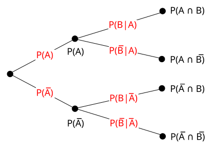
This tree diagram displays sequential events with conditional probabilities on the second-level branches, illustrating how probabilities update when earlier events have occurred. The structure reinforces the meaning of notation such as P(B∣A)P(B \mid A)P(B∣A). The full paths also encode joint probabilities, connecting conditional reasoning to broader probability relationships. Source.

The AP specification emphasizes that conditional probability represents the likelihood of event A occurring given that event B has already occurred, written using the notation P(A | B). This relationship focuses attention on a restricted portion of the sample space—only those outcomes in which event B has taken place.

Conditional probability is essential in statistical reasoning because many real-world situations rely on updated or contextualized information. Instead of considering all possible outcomes, conditional probability narrows the analysis to a subset in which the condition is satisfied.

Why Conditional Probability Matters

Conditional reasoning allows statisticians to incorporate context, new information, and dependencies between events. The specification underscores that conditional probability is not simply a new formula; it is an interpretive shift that changes how we view uncertainty.

Some key motivations for using conditional probability include:

• Focusing on relevant outcomes when certain events have already occurred.

• Reassessing likelihoods when circumstances provide partial information.

• Identifying relationships between events, such as dependence or independence.

• Modeling real-world decision-making, where information evolves over time.

Conditional probability appears in areas such as medical testing, weather prediction, genetics, reliability engineering, and risk analysis. In each of these fields, knowing one event has happened meaningfully alters the likelihood of others.

Mathematical Structure of Conditional Probability

Because conditional probability is based on a restricted sample space, it requires a mathematical structure that reflects this narrowed focus. The probability of “A given B” accounts only for the outcomes in B, measuring the proportion of those outcomes that also fall within A.

EQUATION

When event B has zero probability, the conditional probability P(A | B) is undefined, because no meaningful restriction can be applied. This reinforces the importance of defining events carefully and ensuring that conditions reflect realistic possibilities.

A sentence separating blocks: Conditional probability equations express how probabilities redistribute when additional information is known.

Interpreting the Notation

The notation P(A | B) is read as “the probability of A given B.” The vertical bar represents the idea of conditioning or restricting attention to a particular circumstance. Students should interpret this notation as a signal that:

• We are no longer using the original sample space.

• All outcomes inconsistent with the condition are excluded.

• Probabilities must be recalculated relative to the reduced context.

Understanding this notation prepares students for more advanced probability, including independence, Bayes’ rule, and probability models for real-world processes.

Conceptualizing How Conditioning Works

To conceptualize conditional probability, it often helps to imagine that event B has already happened. Once B is known to occur:

• Every outcome outside of B becomes irrelevant.

• Probabilities are recalculated by looking only within B.

• The likelihood of A depends on how much of B overlaps with A.

This framing highlights that conditional probability is not about adding new information to the original problem but rather about redefining the sample space around event B.

Visual and Structural Thinking

Although these notes do not include diagrams, it is helpful for students to mentally picture Venn diagrams or restricted frequency tables. Visual reasoning reinforces key relationships:

• The region representing A ∩ B corresponds to cases where both events occur.

• The region representing B forms the new sample space.

• The ratio of the overlap to the total area of B conveys the conditional probability.

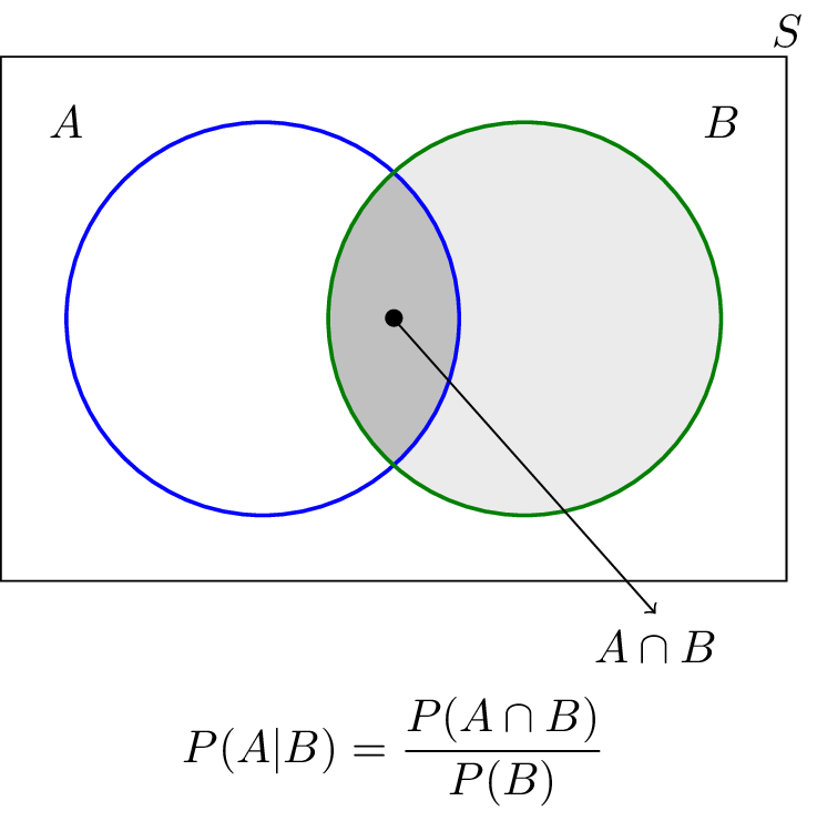
This Venn diagram illustrates events A and B within a sample space, with the intersection A∩BA \cap BA∩B highlighted. It visually demonstrates that conditional probability considers only the outcomes inside B and measures what fraction of those also fall within A. This corresponds directly to the expression P(A∣B)=P(A∩B)P(B)P(A \mid B) = \frac{P(A \cap B)}{P(B)}P(A∣B)=P(B)P(A∩B)​. Source.

Such structural thinking deepens understanding of why P(A | B) fundamentally differs from P(A).

Key Points for AP Statistics

Students should remember the following high-utility ideas aligned with the specification:

• Conditional probability applies when the likelihood of an event changes because new information is available.

• The notation P(A | B) indicates that the probability is calculated under the assumption that B has already occurred.

• Conditional probability focuses on the intersection relative to the condition.

• The concept provides the basis for analyzing statistical dependence and real-world contextual reasoning.

• Understanding conditional probability supports later work with independence, probability rules, and inferential thinking.