
AP Syllabus focus:
‘VAR-4.E.2: Discuss how, for independent events A and B, the probability of both occurring simultaneously, P(A and B), is the product of their individual probabilities, P(A) × P(B). This segment will detail the formula and its application, illustrating the mathematical principle that underpins the calculation of probabilities for independent events.’
This section develops the core principle that independent events allow probability calculations through multiplication, helping students understand how separate random behaviors combine within a single probability framework.
Calculating Probabilities of Independent Events
Understanding Independence in Probability
When working with probability, it is essential to recognize whether two events are independent. Independence determines how their probabilities combine when both are expected to occur in the same scenario. Two events are considered independent when the occurrence of one has no effect on the likelihood of the other. This subsubtopic focuses strictly on how to compute the probability that both events occur, given independence, consistent with the AP Statistics specification.
Independent Events: Two events are independent when the occurrence of one does not affect the probability of the occurrence of the other.
Independence is a structural property of a situation, not something inferred from observed frequencies alone, and it must be clearly identified before applying the multiplication rule.
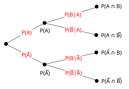
Probability tree diagram showing branching from an initial event into outcomes A and not A, and then B. The labels illustrate how probabilities multiply along each path to form joint probabilities. This focuses on the structure underlying combined events and can be interpreted for independent events when branch probabilities for B remain constant. Source.
The Multiplication Principle for Independent Events
To determine the probability of two independent events A and B occurring together, we multiply their individual probabilities. This is known as the multiplication rule for independent events, and it is central to probability reasoning whenever separate processes or random mechanisms operate without influencing one another.
EQUATION
= Probability that event A occurs (unitless measure between 0 and 1)
= Probability that event B occurs (unitless measure between 0 and 1)
This formula applies only when independence is established. Students must carefully verify independence rather than assuming it based on intuition or superficial pattern recognition.
Conditions Required for Using the Multiplication Rule
To use the multiplication rule properly in AP Statistics:
A and B must be independent, meaning the outcome of one does not change any probability for the other.
Probabilities must be known or well-defined, typically derived from theoretical reasoning or empirical long-run frequencies.
The event of interest must be the joint event A and B, reflecting simultaneous or combined occurrence.
No conditional probability adjustments are needed, unlike dependent events where must account for .
These conditions ensure that multiplying the individual probabilities accurately reflects the underlying random structure.
Interpreting the Probability of Joint Occurrence
The product quantifies how likely both events are to happen in a single combined trial of a process or sequence of processes. This joint probability is always less than or equal to each individual probability because it requires two outcomes to happen rather than one.
When interpreting the result:
The joint probability reflects long-run relative frequency of both events occurring together.
It quantifies how two separate random behaviors combine in repeated trials.
It reinforces the conceptual link between probability and repeated, stable patterns over many observations.
Key Characteristics of Joint Probabilities Under Independence
Several important features follow directly from independence:
The probability of the intersection depends solely on the product of the separate probabilities, not on the order of events.
The size of the probability reflects the compounding effect of requiring two events to occur, typically resulting in a smaller probability.
The multiplication rule remains valid regardless of the context, as long as independence is satisfied.
Independence cannot be inferred merely from low joint probability, since unlikely events may still be dependent structurally.
These characteristics ensure that students understand both the computational aspect and the conceptual depth of independence.
Applying the Rule Within Structured Probability Problems
When analyzing real-world or theoretical probability scenarios, independence must be explicitly identified before applying the multiplication rule. Many settings naturally imply independence, such as outcomes of different rolls of a fair die or results from repeated, identical trials of a random mechanism. Other contexts may require more careful reasoning, even when events appear unrelated.
Students should work through problems by following this structured process:
Identify the events A and B clearly, ensuring their definitions do not overlap in a way that implies dependence.
Confirm independence, either from context or from explicit description.
Determine each individual probability, expressed as a number between 0 and 1.
Multiply the probabilities, using the multiplication rule only after confirming independence.
Interpret the resulting probability, connecting the value to long-run expectations.
Importance of the Multiplication Rule in Statistical Reasoning
The multiplication rule is essential for building understanding in later probability concepts, including random variables, binomial settings, and simulation-based models. It establishes how probability combines across independent components of a process and anchors the logic behind many probability distributions. It also reinforces the principle that independence is a structural assumption tied to context, not simply a computational shortcut.
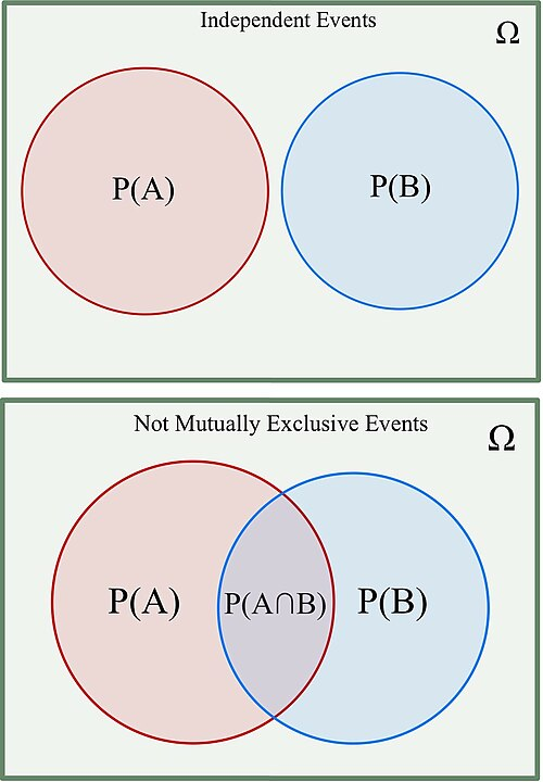
Diagram comparing independent and non-mutually exclusive events through separate and overlapping regions. One panel shows independent events with no shared outcomes, while another displays overlap illustrating non-mutually exclusive relationships. The image includes additional detail on unions of events, which exceeds the syllabus slightly but helps clarify distinctions needed before applying the multiplication rule. Source.
FAQ
Independence is established when knowing the outcome of one event does not change the probability of the other. This usually requires contextual reasoning rather than computation.
Look for cues such as:
• Separate physical processes (e.g., two different machines or random draws with replacement)
• No shared mechanism influencing both outcomes
• Situations where the outcome of one event cannot logically interfere with the other
When the context is ambiguous, independence should never be assumed.
A joint probability requires two outcomes to occur simultaneously, which is a stricter condition than either event occurring alone.
Because of this:
• The probability of both happening can never exceed the chance of the least likely event
• Multiplying probabilities less than 1 always reduces or maintains magnitude
This reflects how combined conditions narrow the set of successful outcomes.
A common mistake is assuming independence from intuition rather than context, especially when events seem unrelated but share a hidden link.
Other misconceptions include:
• Confusing independence with mutually exclusive events
• Believing that independence can be inferred from small joint probabilities
• Forgetting that independence must hold for the specific trial structure described
Clarifying the scenario usually eliminates these errors.
Independence is a strict statistical condition: one event’s occurrence does not change the probability of the other.
“No correlation,” however, is an informal phrase and can mean:
• No visible pattern between events
• No perceived relationship based on casual observation
• A non-mathematical claim that may still involve hidden dependence
Only independence guarantees that probabilities multiply cleanly.
Analysts typically evaluate the mechanism producing each event rather than rely on numerical evidence.
Useful strategies include:
• Mapping out the steps or physical processes producing each outcome
• Checking whether one event alters conditions relevant to the other
• Considering whether the events can be thought of as repeatable identical trials
• Consulting background information about the system generating the events
These methods reduce the risk of assuming independence where it does not hold.
Practice Questions
A retailer reports that the probability a customer uses a discount voucher on a purchase is 0.25. The probability that a customer chooses express delivery is 0.40. The retailer confirms that these two events are independent.
What is the probability that a customer both uses a discount voucher and chooses express delivery on the same purchase? (1–3 marks)
• Uses multiplication rule for independent events: 0.25 × 0.40. (1 mark)
• Correct answer: 0.10. (1 mark)
• Clearly states or implies that independence justifies multiplication, if mentioned. (1 mark)
Maximum 3 marks.
A quality control analyst monitors two independent checks carried out on every item produced in a factory.
• Check A correctly identifies a defect with probability 0.82.
• Check B correctly identifies a defect with probability 0.76.
Let the event that Check A correctly identifies a defect be A, and the event that Check B correctly identifies a defect be B.
(a) State why the multiplication rule can be applied to find P(A and B). (1 mark)
(b) Calculate P(A and B). (2 marks)
(c) Explain what this probability means in the context of repeated quality checks. (1–3 marks)
(a) • States that the events are independent, so the probability of both occurring is the product of their individual probabilities. (1 mark)
(b) • Sets up the calculation: 0.82 × 0.76. (1 mark)
• Correct answer: 0.6232 (or rounded correctly). (1 mark)
(c) • Explains that the value represents the long-run proportion of items for which both checks correctly identify a defect. (1 mark)
• Uses correct contextual language about repeated trials rather than a single instance. (1 mark)
• Provides a clear interpretation such as “In the long run, about 62% of defective items would be correctly identified by both checks.” (1 mark)
Maximum 6 marks.
