
AP Syllabus focus:
‘Introduce the concept of combining random variables, specifically linear combinations. VAR-5.E.1: Explain how the mean of the linear combination of random variables X and Y, with real numbers a and b, is calculated as the sum of a times the mean of X plus b times the mean of Y (μaX+bY = aμX + bμY). This illustrates how means of random variables are combined in linear operations.’
Linear combinations of random variables allow statisticians to describe new variables created through additive or scaled relationships. Understanding how their means interact provides a foundation for analyzing combined random processes.
Mean of Linear Combinations
The study of linear combinations begins with recognizing how operations applied to random variables influence their expected or average outcomes. In this subsubtopic, the focus is on how the mean, also known as the expected value, behaves when random variables are scaled and added together.
A linear combination of random variables is an expression of the form , where and are random variables and and are real-number constants. This construction is central in probability and statistics because many real-world quantities involve multiple uncertain components whose combined behavior must be understood.
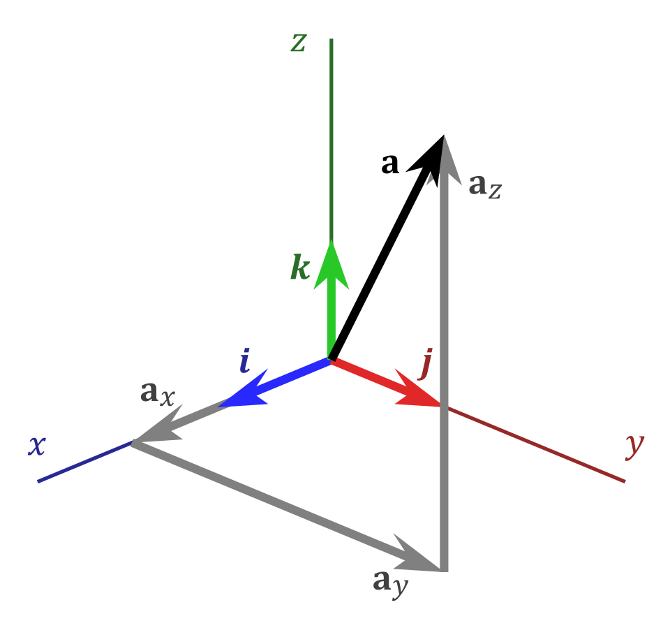
A three-dimensional vector shown as the sum of its component vectors along each axis. This visual analogy illustrates how a single quantity can be constructed from scaled components, mirroring the structure of linear combinations of random variables. The geometric notation exceeds syllabus requirements but reinforces the conceptual idea of combining elements linearly. Source.
Linear Combination of Random Variables: An expression formed by multiplying each variable by a constant and adding the results, written as .
When combining means, the essential idea highlighted by VAR-5.E.1 is that the mean of a linear combination equals the same linear combination of the individual means. This principle allows statisticians to compute the expected value of a newly constructed variable without needing its full probability distribution.
Interpreting Constants in Linear Combinations
The constants and play distinct roles in shaping the new variable.
Multiplying a random variable by a constant stretches or compresses its scale.
Adding scaled random variables merges their behaviors into one combined measure.
These constants directly modify the mean, preserving the structure of linearity.
This behavior demonstrates why expected value is considered a linear operator, meaning it distributes across addition and scalar multiplication in a predictable way.
EQUATION
= Mean of the linear combination
= Real-number constants with no units
= Means of random variables and , using units of their respective variables
Because expected value reflects a long-run average outcome, the combination rule preserves the underlying intuition: scaling a variable scales its average, and adding variables adds their averages.
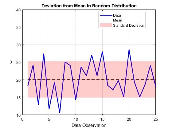
A plotted sequence of random values with a marked mean line and shaded standard deviation region. This illustrates how observations fluctuate around their long-run average, supporting the conceptual basis for understanding expected value. The shading adds extra detail about variability beyond the core syllabus requirement. Source.
A normal sentence must follow to maintain continuity before introducing further structured content. Understanding the influence of constants on the mean helps students interpret how different linear relationships modify the behavior of random variables.
Why Linearity of Expectation Matters
The property captured in VAR-5.E.1 is foundational because it applies to all random variables, regardless of whether they are dependent or independent. This distinguishes the rule for means from rules governing variance, which require independence for similar simplifications. Students should recognize that this generality makes expected value one of the most powerful tools in probability.
Key reasons the linearity of expectation is valuable include:
It simplifies work with large or complex systems.
It avoids needing to compute entire probability distributions.
It applies equally to discrete and continuous random variables.
It enables modeling of totals, differences, and weighted sums.
These features make understanding linear combinations crucial for interpreting combined outcomes in fields such as finance, risk assessment, sampling, and quality control.
Constructing New Variables Using Linear Combinations
A linear combination such as represents a new random variable with its own mean.

Bar chart representing the probability mass function of the sum of two fair dice. Each bar shows the probability of a total from 2 to 12, demonstrating how combining random variables results in a new distribution. Dice icons add extra detail not required by the syllabus but maintain clear educational alignment. Source.
The process of constructing such a variable typically includes the following steps:
Identify the component random variables involved.
Determine the constants representing scaling or weighting.
Express the combined variable algebraically as a linear combination.
Apply the linearity of expectation to compute its mean.
Each step reinforces the idea that the mean behaves predictably under linear operations, supporting deeper statistical modeling later in the course.
A complete understanding of linear combinations provides students with a pathway to analyze more advanced structures, such as weighted averages or aggregated measurements.
Interpreting the Mean of a Linear Combination
Interpreting the mean of requires focusing on the context of the variables. Because the mean always uses the units of the variable being measured, interpreting the combined mean depends on:
The meaning of the constants applied.
How the original variables relate to the phenomenon being modeled.
Whether the linear combination represents a total, a difference, or a transformation.
This ensures students can articulate not only the numerical result but also its statistical meaning within a scenario. Understanding this interpretation aligns with the broader VAR-5 framework, which emphasizes connecting parameters to real-world populations and processes.
Through this subsubtopic, learners develop an essential conceptual tool for analyzing combined random behaviors, setting the stage for later work with variance, independence, and transformations of random variables.
FAQ
A negative constant reverses the direction of the random variable’s scale but still follows the same linear rule for calculating the mean. The constant multiplies the mean directly, even if it is negative.
This does not change how the linearity of expectation works; it simply reduces or inverts the contribution of that variable to the combined mean.
Yes. The principle extends to any finite number of random variables.
If a new variable is formed as a1X1 + a2X2 + … + akXk, the mean is the same combination of individual means:
• Scale each mean by its coefficient
• Add the scaled means together
This remains valid regardless of dependence between the variables.
Yes. The magnitude of each constant indicates how strongly its variable contributes to the combined mean.
Large positive constants increase the influence, whereas small or negative constants reduce or reverse it.
This provides a simple way to interpret weighting schemes in models and indices.
If a variable is rescaled through unit conversion, its mean changes accordingly, and this also affects the combined mean.
For example:
• Converting inches to centimetres multiplies the variable by 2.54
• This scaling applies directly to the variable’s contribution in the linear combination
The linearity of expectation ensures unit conversions behave predictably.
Linearity simplifies complex systems by allowing analysts to calculate expected outputs without deriving full probability distributions.
This is particularly helpful when modelling totals, averages, weighted indices, or composite scores. It reduces computational effort while maintaining accuracy in the expected-value structure.
The property is also fundamental in regression, forecasting, and risk assessment, where multiple uncertain components must be combined.
Practice Questions
Question 1 (1–3 marks)
Two random variables, X and Y, have means of 8 and 3 respectively. A new variable is formed as T = 2X + Y.
(a) State the mean of T.
(b) Give a brief reason why this calculation does not require knowledge of the full probability distributions of X and Y.
Question 1
(a) Mean of T
• Correct substitution: 2(8) + 3
• Correct final answer: 19
(1 mark)
(b) Reasoning
• States that the expected value is linear OR that the mean of a linear combination equals the same linear combination of the means.
• Notes that this property does not depend on the underlying distributions.
(1–2 marks)
Total: 2–3 marks
Question 2 (4–6 marks)
A researcher measures the heights of plants grown under two different conditions. Let H represent the height (in cm) of a plant grown in sunlight, with a mean of 42 cm. Let S represent the height (in cm) of a plant grown in shade, with a mean of 35 cm.
The researcher creates a combined growth score defined as G = 1.5H − 0.5S.
(a) Calculate the mean of G.
(b) Explain why the mean of G can be calculated even if H and S may be related.
(c) Interpret the meaning of the mean of G in the context of plant growth.
Question 2
(a) Calculation
• Correct method: 1.5(42) − 0.5(35)
• Correct final answer: 41.5
(2 marks)
(b) Explanation
• States that linearity of expectation applies regardless of whether H and S are dependent or independent.
(1–2 marks)
(c) Interpretation
• Identifies that the value represents the long-run average combined growth score.
• Relates the score to the weighted contribution of sunlight- and shade-grown plants in a biological context.
(1–2 marks)
Total: 4–6 marks
