
AP Syllabus focus:
‘VAR-5.E.3: Detail the formula for calculating the variance of the linear combination of independent random variables X and Y with real numbers a and b, showing that the variance is the sum of the square of a times the variance of X plus the square of b times the variance of X (σ^2aX+bY = a^2σ^2X + b^2σ^2Y). This subsubtopic explains how variances add, even when random variables are linearly combined, given they are independent.’
This section introduces how variance behaves when random variables are combined linearly, highlighting how independence allows variances to add in a predictable mathematical structure.
Variance in the Context of Linear Combinations
Understanding the variance of linear combinations is essential for describing how uncertainty accumulates when multiple random variables are combined. In statistics, the behavior of variance is especially important because it determines the spread of possible values for combinations such as totals, differences, and scaled variables. This subsubtopic focuses on how variance changes when two independent random variables are combined using real-number multipliers.
Linear Combinations of Random Variables
A linear combination involves forming a new random variable using constants and existing variables, written in the general form aX + bY, where a and b are real numbers. When examining the variability of such a combination, the goal is to determine how each component contributes to the overall spread of the resulting distribution. Because variance measures the average squared deviation from the mean, it reflects how much uncertainty is introduced by each part of the linear expression.
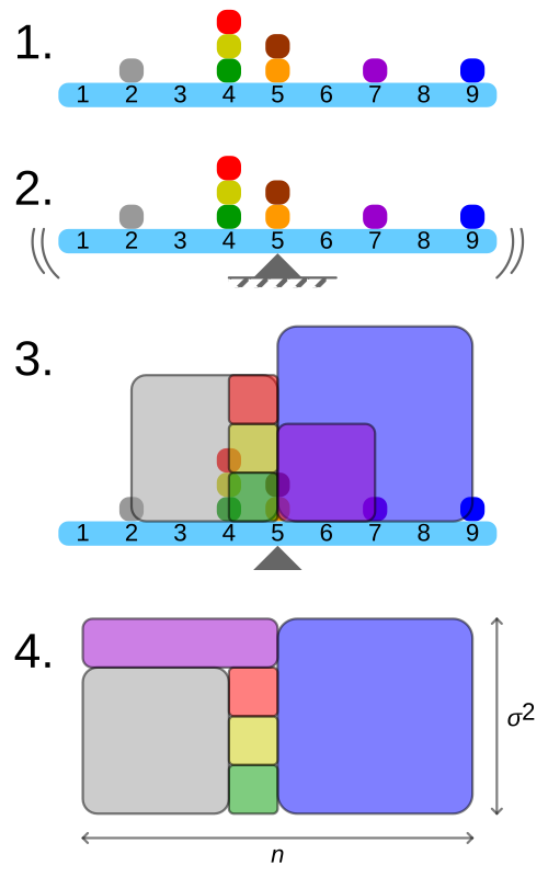
This figure shows a frequency distribution for a small data set, the location of the mean, and squares whose areas represent the squared deviations from that mean. Rearranging the squares into a rectangle highlights how the total area corresponds to the variance, emphasizing variance as an average of squared distances from the mean. The specific numerical example and exact data values extend beyond this subsubtopic but strengthen conceptual intuition for variance. Source.
Why Independence Matters
The AP syllabus requires understanding that the variance formula presented in this subsubtopic applies only when X and Y are independent random variables, meaning knowledge about the outcome of one does not provide information about the other.
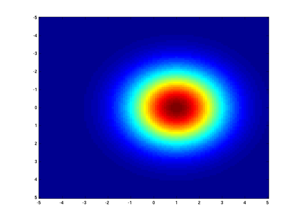
This scatterplot displays samples from a bivariate normal distribution with independent coordinates and equal variance in both directions, forming an approximately circular cloud. The lack of directional pattern or tilt illustrates independence: knowing the value on one axis does not help predict the value on the other. The specific distribution shown is more general than required for AP Statistics but effectively demonstrates independence and equal spread. Source.
Independent Random Variables: Random variables X and Y for which the outcome of one does not influence the probability distribution of the other.
Independence guarantees that the variability contributed by each variable is separate and can be analyzed individually, allowing the variance of their combination to be determined by examining each component in isolation before combining them.
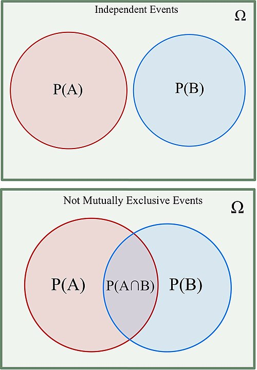
This figure contrasts independent events, shown with no overlap, and non-mutually-exclusive events, shown with overlapping circles. The non-overlapping case supports the idea that independent structures contribute separately to probability calculations, paralleling how independent variables contribute separately to variance. The panel showing non-mutually-exclusive events exceeds this subsubtopic’s scope but can be ignored when focusing strictly on independence. Source.
Structure of Variance in Linear Combinations
When forming the linear combination aX + bY, each constant affects the scale of its corresponding variable. Scaling a random variable affects variance differently than scaling affects the mean. Because variance is based on squared deviations, multiplying a variable by a constant multiplies its variance by the square of that constant. This squared scaling effect is at the center of the AP-required variance formula.
EQUATION
= Variance of the linear combination aX + bY
= Real-number multiplier applied to X
= Variance of random variable X
= Real-number multiplier applied to Y
= Variance of random variable Y
This equation demonstrates that the contributions to total variance come from each variable independently, with each contribution adjusted by the square of its coefficient. Because the variables are independent, their variances combine additively.
A variable must appear as a squared term in the formula to reflect how spread changes under scaling. This feature ensures that variance always remains non-negative and that increases in magnitude of a or b proportionally increase the uncertainty in the resulting combination.
Interpreting the Variance Formula
Interpreting the variance of a linear combination requires recognizing how each part of the equation corresponds to a statistical effect:
a²σ²X shows how the variability of X increases when X is stretched or compressed by factor a.
b²σ²Y shows how the variability contributed by Y changes under scaling by b.
Addition of the two terms reflects the idea that when variables do not interact probabilistically, their uncertainties accumulate.
The additive nature of variance under independence makes linear combinations predictable and analytically useful. For example, summing many independent variables produces increasing variance, growing in proportion to the number of terms and the square of any scaling constants used.
Key Features of Variance in Linear Combinations
Students should understand several essential principles derived from the syllabus requirement:
Variance measures spread, not central tendency, so linear combinations change variance differently from how they change means.
Independence ensures that the variability added by one variable is unaffected by the other.
Scaling factors modify variance through squares, emphasizing the sensitivity of variance to magnitude changes.
The final variance of a combination reflects the cumulative uncertainty contributed individually by each random variable.
These ideas reinforce why variance plays a central role in probability distributions and why understanding its behavior under linear combinations is foundational in AP Statistics.
FAQ
If a coefficient is zero, the corresponding random variable contributes no variance to the linear combination. The variable is effectively removed from the expression.
This is because variance scales with the square of the coefficient, and zero squared is zero.
In such cases, the variance of the linear combination is simply the variance of the remaining term(s) adjusted by their squared coefficients.
Squared coefficients appear because variance measures the average squared distance from the mean. When a random variable is scaled by a constant, each deviation from the mean is also scaled, and squaring these deviations results in the coefficient being squared.
This ensures variance reflects both the magnitude of the scaling and the spread of the original variable.
Yes. A linear combination can have smaller variance than either individual variable, depending on the coefficients.
For example:
• Negative coefficients can counteract variability between terms.
• Smaller coefficients (fractions) reduce overall spread.
Because variance is sensitive to scaling, reducing the magnitude of coefficients reduces the total variability.
Yes, but only in very specific situations. A linear combination has zero variance when it produces a constant value with no randomness.
In the context of independent variables, this occurs only if the linear combination cancels out all variability exactly, which requires carefully chosen coefficients and identical distributions.
In practice, such cancellations are rare in real-world data.
The shape of the distribution does not change how variance combines in linear combinations, provided the variables are independent.
However, the shape can influence how meaningful or useful the resulting variance is for interpretation.
• Skewed distributions may produce linear combinations with asymmetric behaviour.
• Heavy-tailed distributions may lead to unusually large variance values.
The combining rule remains the same regardless of distribution shape.
Practice Questions
Question 1 (1–3 marks)
A random variable X has variance 9, and a random variable Y has variance 4. The variables X and Y are independent.
Calculate the variance of the linear combination 2X − 3Y.
(3 marks)
Mark scheme for Question 1
• Correct use of the rule Var(aX + bY) = a²Var(X) + b²Var(Y) for independent variables (1 mark)
• Correct substitution: 2²(9) and (−3)²(4) (1 mark)
• Correct final answer: 36 + 36 = 72 (1 mark)
Question 2 (4–6 marks)
A researcher is analysing two independent random variables:
• X, representing daily demand for a product (in units), with variance 25
• Y, representing the number of defective items in a shipment, with variance 9
The researcher models the total number of items that will need to be replaced as T = 3Y − X.
(a) Show how the variance of T is calculated.
(b) Compute the variance of T.
(c) Briefly explain why independence is important in this calculation.
(6 marks)
Mark scheme for Question 2
(a) States the formula for the variance of a linear combination of independent variables: Var(aX + bY) = a²Var(X) + b²Var(Y) (1 mark)
Correctly applies the coefficients: Var(T) = (−1)²Var(X) + 3²Var(Y) (1 mark)
(b) Correct substitution: Var(T) = 1(25) + 9(9) (1 mark)
Correct calculation: 25 + 81 = 106 (1 mark)
(c) Explains that independence ensures no covariance term is required (1 mark)
States that without independence, the variances would not simply add and an extra term involving the relationship between X and Y would be needed (1 mark)
