
AP Syllabus focus:
‘Calculate the probability that a particular value lies within a given interval of a normal distribution. This involves understanding continuous random variables, which can take on any value within a specified domain. It's crucial to recognize that every interval within the domain has a probability associated with it. A continuous random variable with a normal distribution describes populations with a bell-shaped curve. The area under a normal curve over a given interval signifies the probability of a particular value lying within that interval.’
Understanding how to calculate probabilities within a normal distribution allows statisticians to quantify uncertainty, interpret population patterns, and make meaningful inferences about continuous random variables.
The Normal Distribution and Continuous Random Variables
A continuous random variable is a variable that can take on any value within a specified domain.
Continuous Random Variable: A variable that assumes infinitely many possible values within a given interval, each associated with a probability determined by an underlying distribution.
The normal distribution is one of the most important continuous distributions in statistics because many real-world measurements follow approximately bell-shaped patterns. When a variable is normally distributed, probabilities correspond directly to areas under its smooth, symmetric curve.
Key Characteristics of the Normal Curve
The normal curve is centered at its mean, with its spread determined by the standard deviation.
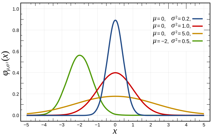
Multiple normal curves illustrating how changes in mean and variance shift or stretch the distribution. Extra detail: several curves are shown, though AP Statistics typically focuses on one distribution at a time. Source.
These parameters define the shape and behavior of the distribution. Importantly, every possible interval under this curve carries an associated probability, making interval-based reasoning essential in probability calculations.
EQUATION
= Standardized value (z-score)
= Observed value of the variable
= Mean of the distribution
= Standard deviation of the distribution
Standardizing a value using a z-score converts it to the standard normal distribution, enabling the use of probability tables or technological tools to determine areas under the curve.
Interpreting Probability as Area
The crucial idea in this subsubtopic is that probability equals area under the normal curve over a specified interval.
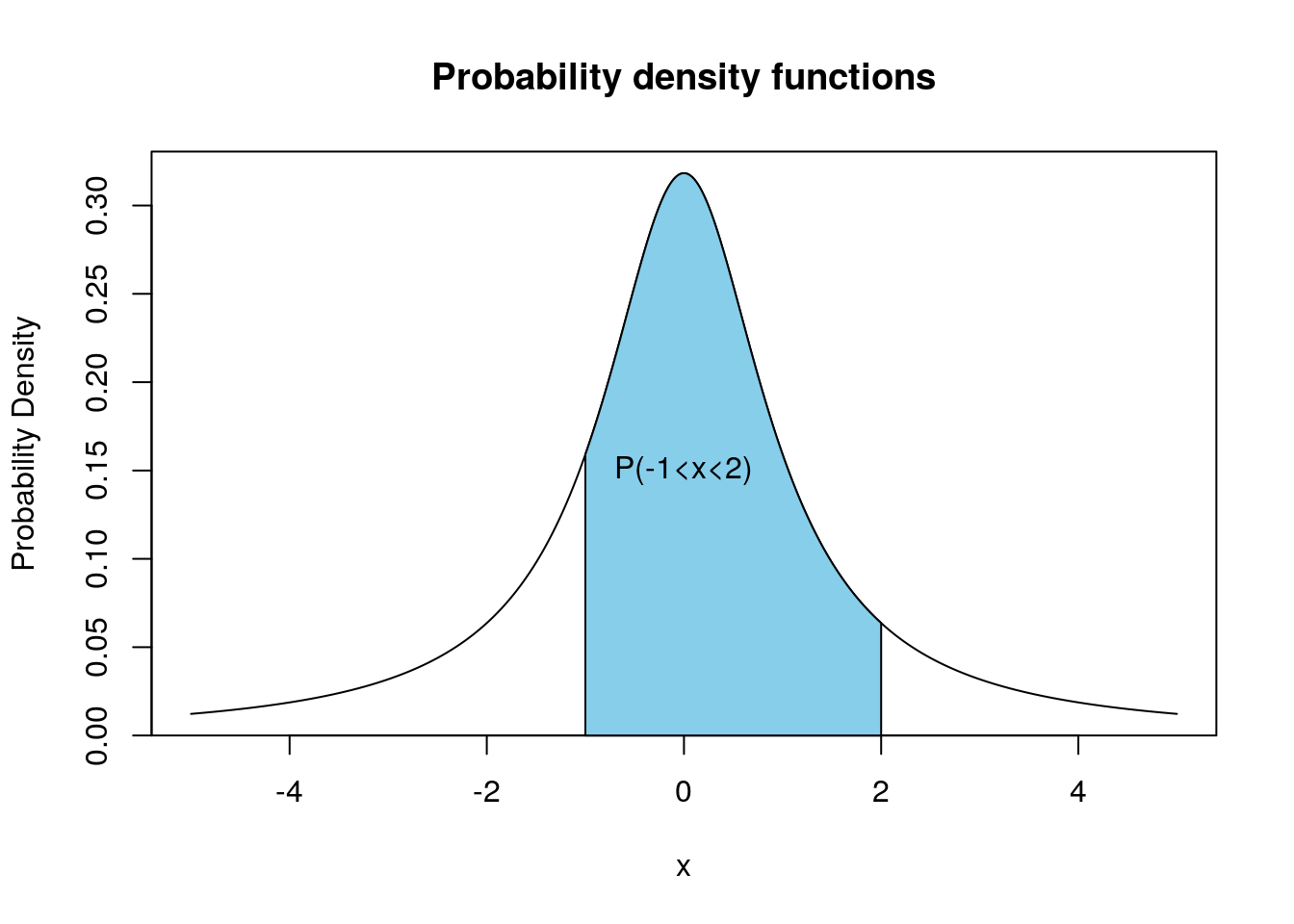
A shaded interval on a density curve showing that probability corresponds to area under the curve. Extra detail: the specific bounds −1 and 2 are simply an example and not required by the AP syllabus. Source.
Since the curve represents a continuous distribution, the total area under it equals 1. This property ensures that all probabilities fall between 0 and 1 and sum to the whole distribution.
Probability questions about normally distributed variables typically ask:
The probability that the variable falls above a value.
The probability that the variable falls below a value.
The probability that the variable lies between two values.
Regardless of the question, calculating the probability always corresponds to finding the area under the curve for that specific interval.
The Role of the Standard Normal Distribution
To calculate probabilities efficiently, statisticians use the standard normal distribution, which has mean 0 and standard deviation 1. Transforming any normally distributed variable into a standardized one allows the use of widely available resources such as:
Standard normal (z-score) tables
Statistical calculators
Computer-generated output
These tools provide the area under the curve to the left of any given z-score.
For example, to find the probability that a value falls between two points, one subtracts the area to the left of the lower boundary from the area to the left of the upper boundary. This approach relies on the fact that probabilities accumulate from the far left of the distribution.
Understanding Intervals in Probability Calculations
When working with the normal distribution, intervals correspond to precise probability statements:
Lower-tail probabilities: The probability that a value lies to the left of a given point.
Upper-tail probabilities: The probability that a value lies to the right.
Middle probabilities: The probability that the value lies within two boundaries.
These interpretations rely on the continuity of the distribution. Because continuous distributions do not assign probability to individual points, all meaningful probability statements involve intervals, not single outcomes.
Normal Distribution: A continuous, symmetric, bell-shaped probability distribution fully described by its mean and standard deviation, used to model many natural and social processes.
The continuous nature of the normal curve ensures that probability statements reflect ranges of values rather than isolated points.
Using Technology to Determine Probabilities
Modern statistical practice often uses tools capable of computing areas under the normal curve instantly. These technological tools include:
Graphing calculators (normalcdf functions)
Spreadsheet software
Statistical packages
Online normal distribution calculators
They allow students and analysts to bypass manual table lookups while preserving the conceptual requirement: probability equals area under the curve for a specified interval.
Practical Interpretation of Normal Probabilities
When interpreting a probability derived from a normal distribution, it is essential to consider:
The context of the variable (e.g., heights, reaction times).
The units of measurement tied to the original distribution.
The meaning of the probability value (e.g., likelihood, proportion of population).
These contextual considerations ensure that probabilities derived from the normal distribution meaningfully relate back to real populations and real data.
The ability to connect interval areas to meaningful probability statements forms the foundation for later inferential methods in AP Statistics, making this subsubtopic crucial to the broader study of sampling distributions and statistical reasoning.
FAQ
When an interval lies very close to the mean, the probability is relatively large because the mean is the point of highest density in a normal distribution.
Small changes near the mean can noticeably shift probability, as a large portion of the total area lies close to the centre.
If the interval straddles the mean, the probability will include equal contributions from both sides of the distribution due to symmetry.
The height of the curve represents density, not probability. Density indicates how tightly values cluster around a point, but it does not assign probability to that point itself.
Probability comes only from the area under the curve. Since a single point has no width, its area is zero, and therefore its probability is zero.
Intervals that align with commonly known z-score areas are easiest to estimate, such as one standard deviation from the mean.
Intervals become harder when:
• boundaries lie at unusual z-scores
• the interval is extremely narrow
• the interval lies far in the tails, where probabilities are very small
Symmetry around the mean often helps simplify mental estimation.
Upper-tail probabilities measure the likelihood of observing unusually large values, whereas lower-tail probabilities measure the likelihood of unusually small values.
These tails correspond to the extremes of the distribution, where probability decreases rapidly.
Tail probabilities are often used to identify rare or exceptional outcomes in continuous data.
Standardising removes the original measurement units, placing all values on a common scale centred at zero.
This allows comparisons between variables with different means and spreads.
For example, a z-score of 2 in any normal distribution indicates a value two standard deviations above the mean, regardless of the variable’s original units.
Practice Questions
Question 1 (1–3 marks)
A variable X is normally distributed with mean 80 and standard deviation 6.
Calculate the probability that X is less than 74. Give your answer to three decimal places.
Question 1 (3 marks)
• 1 mark: Correct z-score calculation for 74 using z = (74 − 80) / 6.
• 1 mark: Identification of area to the left of the calculated z-score.
• 1 mark: Correct probability to three decimal places (approximately 0.091).
Question 2 (4–6 marks)
The reaction time of athletes in a training programme is modelled by a normal distribution with mean 0.42 seconds and standard deviation 0.07 seconds.
a) Calculate the z-score for a reaction time of 0.50 seconds.
b) Hence determine the probability that a randomly selected athlete has a reaction time greater than 0.50 seconds.
c) Explain, in context, what this probability means.
Question 2 (6 marks)
a) (2 marks)
• 1 mark: Correct substitution into z = (x − mean) / standard deviation.
• 1 mark: Correct z-score (approximately 1.14).
b) (2 marks)
• 1 mark: Correct identification that the probability required is the upper tail (1 − area to the left of the z-score).
• 1 mark: Correct probability (approximately 0.127).
c) (2 marks)
• 1 mark: A clear contextual interpretation, e.g., “About 12.7% of athletes have reaction times slower than 0.50 seconds.”
• 1 mark: Correct reference to interpreting probability as a proportion of the population.
