Assessing the normality of the sampling distribution of p-hat is essential for constructing valid confidence intervals, ensuring that inference procedures appropriately model the behavior of sample proportions.

Assessing Sample Distribution Normality

A central requirement for using a one-sample z-interval for a population proportion is verifying that the sampling distribution of the sample proportion, denoted p-hat, is approximately normal. This subsubtopic focuses on determining when this normal approximation is justified, based on the size and composition of the sample. Normality is vital because the z-interval relies on the assumption that the sampling distribution behaves like a normal distribution, enabling the use of critical values from the standard normal model.

Why Normality Matters for p-hat

When constructing a confidence interval for a population proportion, students assume that repeated random samples of size n generate sample proportions whose distribution is approximately normal. This shape allows us to model variation using familiar properties of the normal distribution and to compute margins of error with standard methods. However, this approximation is only appropriate when the sample contains sufficient evidence—through counts of both successes and failures—that the normal model behaves reliably.

Understanding p-hat and the Sampling Distribution

The sample proportion p-hat represents the proportion of individuals in the sample who fall into the category of interest. Because p-hat varies from sample to sample due to sampling variability, its distribution must be reasonably well-behaved to support the inference process. When the normality condition fails, the sampling distribution becomes skewed, and confidence interval calculations may be inaccurate.
When the normality condition holds, the histogram of p-hat from many random samples is unimodal, symmetric, and well-approximated by a normal curve centered at the true population proportion.

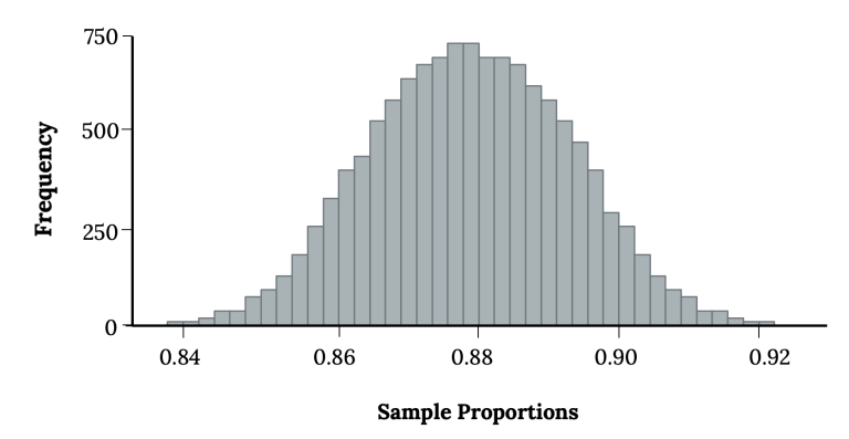
Histogram of a simulated sampling distribution of p-hat from 10,000 samples, showing a symmetric, bell-shaped curve when normality conditions are satisfied. Source.

After introducing the sampling distribution, it becomes important to identify when this distribution resembles a normal curve closely enough for z-based methods.

The Normality Condition Using Counts of Successes and Failures

To assess normality, AP Statistics requires checking whether the sample includes enough successes and failures. Specifically, students verify two inequalities based on the observed sample proportion.

EQUATION

Meeting these conditions indicates that the sampling distribution of p-hat is approximately normal, according to the Central Limit Theorem for proportions, which states that with sufficiently large sample counts, the distribution becomes nearly normal regardless of the population shape.

Interpreting the Counts: Successes and Failures

To apply the condition, the sample must contain both:

• At least 10 successes, meaning the number of individuals in the sample possessing the characteristic of interest is sufficiently large.

• At least 10 failures, meaning the number of individuals not possessing the characteristic is also sufficiently large.

These thresholds ensure that neither tail of the sampling distribution is excessively thin or distorted.

When the Normality Condition Fails

If either np-hat or n(1 − p-hat) falls below 10:

• The sampling distribution becomes skewed, often toward the side of the smaller count.

• The margin of error computed using normal methods may be misleading.

• The resulting confidence interval may misrepresent the uncertainty in the estimate.

When np-hat or n(1 − p-hat) is small, especially when the true proportion is near 0 or 1, the sampling distribution can be strongly skewed and far from normal.

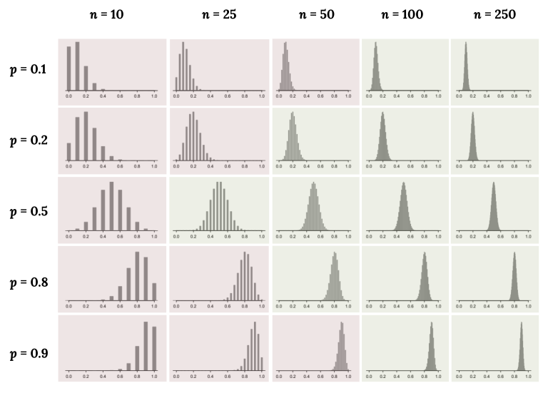
Grid of sampling distributions illustrating how extreme p values or small sample sizes create skewed, non-normal shapes, while larger expected counts yield distributions that approach normality. Source.

In these situations, alternative methods—such as exact binomial procedures—may be preferred, though such methods are beyond the scope of AP Statistics.

Practical Steps for Students

When assessing sample distribution normality as part of constructing a confidence interval, students typically follow this process:

• Identify p-hat.
  Use sample data to compute the observed proportion.

• Compute expected counts.
  Multiply the sample size by p-hat and by (1 − p-hat).

• Check for adequacy.
  Confirm that both values meet or exceed the threshold of 10.

• Validate normality.
  Only proceed with the one-sample z-interval if the condition is met.

As n increases while p stays the same, the sampling distribution of p-hat becomes more tightly concentrated around p and more closely resembles a normal curve.

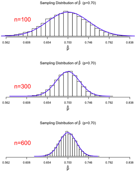
Three sampling distributions of p-hat for increasing sample sizes, demonstrating that larger n values produce narrower, more normal-shaped distributions consistent with the success–failure condition. Source.

Connecting Normality to Reliable Inference

Because inference for proportions depends on approximating p-hat’s distribution with a normal curve, this condition directly affects the accuracy of interval estimates. The strength of the normal approximation ensures that the critical value (z)*, standard error, and margin of error accurately quantify uncertainty. When the approximation is valid, students can trust that their confidence interval is properly calibrated and interpretable.

Thus, assessing sample distribution normality is not a procedural formality—it is the foundation for making justified and statistically sound inferences about population proportions using confidence intervals.