
AP Syllabus focus:
‘Probability of a Type I Error (α): The significance level set before conducting the test. It represents the probability of rejecting the null hypothesis when it is, in fact, true.
- Probability of a Type II Error: Complement of the test’s power (1 - power). The power of a test is the likelihood of correctly rejecting a false null hypothesis.’
Understanding how to calculate the probabilities of Type I and Type II errors is essential for evaluating the reliability of conclusions drawn from significance tests involving population proportions.
Calculating the Probability of Type I and Type II Errors
Understanding Error Probabilities in Statistical Testing
In hypothesis testing for population proportions, every decision carries the risk of error because conclusions rely on sample data subject to random sampling variability. The probabilities associated with these errors help quantify the likelihood of making incorrect decisions when interpreting statistical evidence. These probabilities are central to evaluating how strict or lenient a test should be when determining whether results meaningfully contradict the null hypothesis.
A Type I Error occurs when a true null hypothesis is mistakenly rejected. A Type II Error occurs when a false null hypothesis is not rejected. Both probabilities guide how researchers balance caution and sensitivity in decision-making.
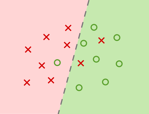
Illustrates the four possible decision outcomes in a binary classification context, with false positives and false negatives aligning conceptually with Type I and Type II errors. Additional labels such as precision and recall are present, extending beyond the syllabus but providing broader decision-framework context. Source.
Type I Error: Rejecting the null hypothesis when the null hypothesis is actually true.
A Type I Error is controlled directly by the significance level, denoted α, chosen before conducting the test.
Significance Level (α): The predetermined probability of making a Type I Error when performing a hypothesis test.
When α is set (commonly 0.05), the researcher explicitly chooses the probability of rejecting a true null hypothesis. Because α is not calculated from data but rather specified, the “probability of a Type I Error” is always equal to α for a properly conducted test.
How α Determines the Probability of a Type I Error
The probability of a Type I Error arises from the rejection region established by the critical value associated with α. In a one-sample z-test for a proportion, more extreme observed test statistics fall in the rejection region. By setting α:
A smaller α reduces the likelihood of a Type I Error but makes rejection of the null hypothesis harder.
A larger α increases the likelihood of a Type I Error but makes it easier to detect possible effects.
These trade-offs highlight why α reflects a balance between the risk of false positives and the need for sensitivity to meaningful differences.
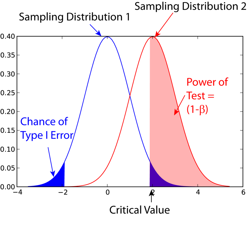
Displays the null and alternative distributions with clearly marked rejection regions, the Type I error probability (α), and the power (1 − β). This visualization supports understanding of how α and power arise from the critical cutoff. Source.
Understanding the Probability of a Type II Error
A Type II Error occurs when a test fails to detect a false null hypothesis. Unlike α, this probability cannot be directly set. Instead, it depends on the true population proportion, sample size, and significance level.
Type II Error: Failing to reject the null hypothesis when the null hypothesis is actually false.
The probability of a Type II Error is represented by β. Because β depends on unknown population conditions, it cannot be directly controlled without adjusting study design features.
Power of a Test: The probability of correctly rejecting a false null hypothesis.
Since power reflects the ability to detect real effects, it relates directly to Type II errors through:
EQUATION
= Probability of a Type II Error
A complete understanding of error probabilities helps explain how changes in study design influence the strength of statistical conclusions.
Factors Influencing the Probability of Type II Error
The size of β is shaped by several structural characteristics of the test:
Sample size (n): Larger samples produce less variability in the sampling distribution, reducing β and increasing power.
True distance between the actual proportion and the hypothesized proportion: Larger differences are easier to detect, reducing β.
Significance level (α): Increasing α widens the rejection region, decreasing β but raising the likelihood of a Type I Error.
Standard error magnitude: Smaller standard errors create tighter sampling distributions, making departures from the null easier to detect.
Because these factors determine how easily a test identifies true differences, researchers often adjust one or more of them to achieve a desired level of reliability.
Balancing Type I and Type II Error Probabilities
The probabilities of Type I and Type II errors are inherently connected. Reducing one typically increases the other unless compensatory adjustments are made. For example:
Lowering α reduces the chance of a Type I Error but increases β unless the sample size is increased.
Increasing sample size simultaneously reduces both error probabilities by lowering overall sampling variability.
A meaningful effect size, when present, naturally lowers β because the observed result is more likely to fall in the rejection region.
Understanding these relationships ensures that statistical tests are designed to meet the goals of a study, whether prioritizing caution against false positives or sensitivity to actual effects.
Interpreting Error Probabilities in Context
Proper interpretation requires linking these probabilities to real study consequences. A Type I Error might incorrectly suggest a meaningful difference in a population proportion, while a Type II Error might obscure one. The choice of α and the design decisions that influence β should be guided by the relative seriousness of each type of mistake in context, reflecting scientific, ethical, or practical priorities of the research scenario.
FAQ
Larger samples produce sampling distributions with smaller standard errors, making the null and alternative distributions narrower. This reduces the overlap between them, decreasing the probability of a Type II error while leaving the Type I error fixed at the chosen significance level.
Smaller samples create wider distributions that overlap more, making it harder to distinguish between the null and alternative hypotheses.
Yes, but usually only by increasing sample size. Since reducing the significance level lowers Type I error but increases Type II error, both can be improved simultaneously only through design choices that reduce variability.
• Increasing sample size is the most effective method.
• Improving measurement precision may also help in some contexts.
The true effect size refers to how far the actual population proportion is from the hypothesised value. Larger differences are easier to detect, reducing the probability of a Type II error.
Smaller effect sizes require larger samples; otherwise, the test may not have enough power to identify meaningful deviations from the null hypothesis.
A one-sided test allocates the entire significance level to one tail, increasing sensitivity to departures in that direction and reducing the chance of a Type II error for that direction.
However, if the true effect is in the opposite direction, the likelihood of a Type II error increases substantially.
The probability of a Type II error depends on the unknown true population proportion, which cannot be specified before observing data.
Because different true values lead to different sampling distributions, β cannot be assigned a single value without assuming a specific alternative. Instead, power analyses evaluate β under chosen plausible alternatives.
Practice Questions
(1–3 marks)
A researcher conducts a hypothesis test at a significance level of 0.05. Explain what this significance level represents in terms of Type I error.
(1–3 marks)
• 1 mark: Identifies that the significance level is the probability of rejecting the null hypothesis when it is actually true.
• 1 mark: States explicitly that this corresponds to the probability of committing a Type I error.
• 1 mark: Notes that at a 0.05 significance level, there is a 5% chance of such an incorrect rejection.
(4–6 marks)
A company claims that 60% of customers prefer its new product. A hypothesis test is carried out at the 5% significance level. Assume that in reality only 55% of customers prefer the product.
a) State what a Type II error would be in this context.
b) Explain two factors that could reduce the probability of making a Type II error in this situation.
c) Briefly describe what the power of this test represents in the context of the company’s claim.
(4–6 marks)
a) (1–2 marks)
• 1 mark: States that a Type II error is failing to reject the null hypothesis when it is false.
• 1 mark: Interprets this in context (e.g., concluding that 60% prefer the product when in reality only 55% do).
b) (2–3 marks)
Award up to 2 marks for any two correct explanations:
• Increasing the sample size reduces sampling variability, decreasing the chance of missing the true difference.
• Increasing the significance level widens the rejection region, reducing the chance of failing to reject a false null hypothesis.
• A larger difference between the true proportion and the hypothesised proportion would make the alternative easier to detect.
Each correct factor with explanation earns 1 mark (max 2).
An additional mark may be awarded for clear, well-linked reasoning.
c) (1 mark)
• 1 mark: States that the power of the test is the probability of correctly rejecting the null hypothesis when it is false, interpreted in context (detecting that fewer than 60% actually prefer the product).
