
AP Syllabus focus:
‘- Relationship between variables may be linear, with y = a + bx as the sample line estimating the population line µy = α + βx.
- Residuals (yi - y^i) estimate deviations from the population regression line.
- The slope of the sample regression line b is unbiased for the population slope β, with its variability quantified by standard error.
- A t-interval is appropriate for estimating the slope's confidence interval.’
Identifying an Appropriate Confidence Interval Procedure
Understanding when and how to construct a confidence interval for a regression slope is essential for assessing uncertainty in linear relationships and estimating population parameters responsibly.
The Purpose of Confidence Intervals for a Regression Slope
Confidence intervals for slopes help quantify uncertainty when using a sample to estimate the population slope (β) in a linear relationship. Because sample data vary randomly, each sample produces a slightly different estimate of the slope, meaning that the observed slope (b) cannot perfectly represent the population. A confidence interval provides a range of plausible values for β, reflecting both sample variation and model assumptions.
Understanding the Regression Model Structure
In simple linear regression, a sample is used to estimate the underlying population relationship between two quantitative variables. The sample regression line is written as , serving as an estimate of the population regression line .
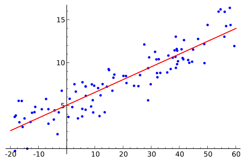
A scatterplot showing sample data with a fitted regression line, illustrating how a sample line estimates the population regression line in simple linear regression. Source.
Sample Slope (b): The estimated rate of change in the response variable for each unit change in the explanatory variable, calculated from sample data.
Because sample slopes vary from sample to sample, they form a distribution centered around the true population slope.
A crucial feature of regression analysis is the residual, the difference between an observed value and its predicted value.
Residual (): The deviation between an observed response value and the value predicted by the sample regression line.
Residuals give insight into how well the sample line represents the population line and provide important diagnostic information about model fit.
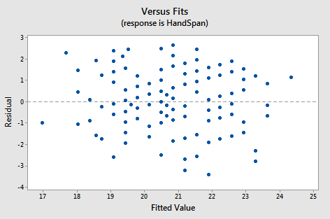
A residual plot showing random scatter around zero with roughly constant spread, indicating that linearity and constant variance conditions are reasonably satisfied. Source.
Why the Slope Estimate Has Variability
The slope estimator b is considered unbiased, meaning its expected value equals the population slope β. However, the amount of variability in b depends on sample size and data dispersion. This variability is summarized by the standard error of the slope, which reflects how much sample slopes fluctuate across repeated samples.
EQUATION
= Standard error of the slope, measuring variability
= Standard deviation of residuals
= Individual explanatory variable value
= Mean of explanatory variable values
This measure plays a central role in determining an appropriate interval estimate.
A sentence of explanation fits here to maintain spacing requirements.
Recognizing When a t-Interval Is Appropriate
For slope inference, a t-interval must be used rather than a z-interval. This choice is required because the standard error comes from sample data rather than the population, meaning the sampling distribution of the slope follows a t-distribution with n − 2 degrees of freedom when regression assumptions hold.
A t-interval becomes the correct procedure when the goal is to estimate the population slope β and the regression conditions are reasonably satisfied. Because the slope’s sampling distribution depends on unknown variability estimated from the sample, the t-distribution accounts for added uncertainty, especially for smaller samples.
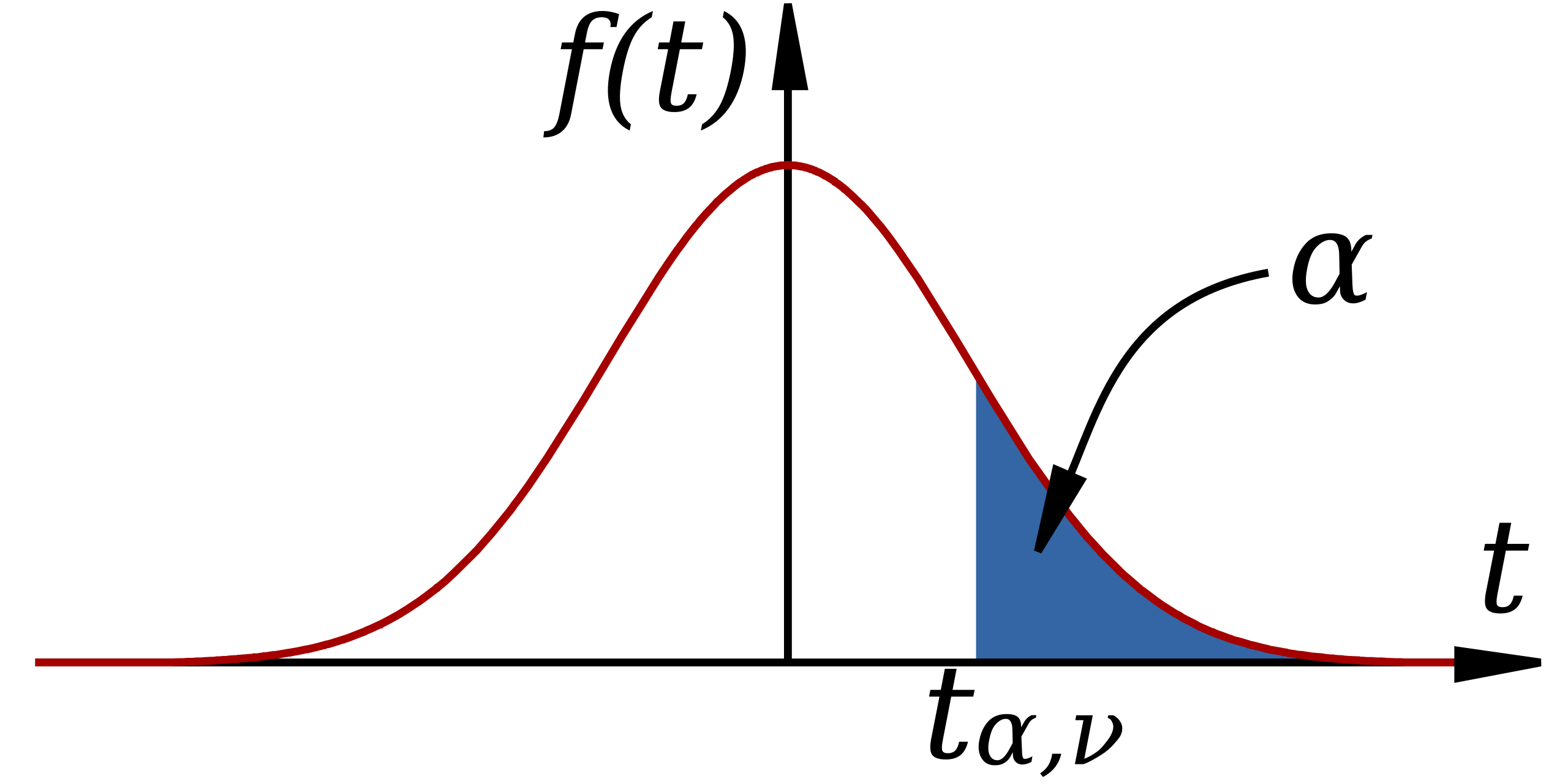
A t-distribution curve with a highlighted critical value, illustrating how t∗t^*t∗ defines the tail probability used when constructing a confidence interval for the slope. Source.
Components Required for Identifying the Procedure
To determine that a t-interval is the correct method, a student should check that:
The research question involves estimating the population slope β.
A linear regression model is appropriate for describing the relationship.
The slope estimate b comes from a sample drawn using proper data-collection methods.
The standard error of the slope is available or can be computed from regression output.
Conditions for inference—linearity, independence, constant variability, and normality of residuals—are at least approximately met.
Identifying these components ensures valid estimation and guards against misinterpretation.
Why Confidence Interval Identification Matters
Using the appropriate interval procedure helps contextualize uncertainty in real-world relationships. A t-interval for β does not simply estimate a slope; it reflects how strongly the sample supports the existence and direction of a linear association. Recognizing this purpose allows students to distinguish between descriptive sample patterns and inferential statements about populations.
The Role of Residuals in Confirming Appropriateness
Residuals serve as the key diagnostic tool for determining whether slope inference procedures can be used. By inspecting patterns in residual plots, analysts assess whether deviations appear random or exhibit a systematic pattern, which would signal a poor model fit. Since the interval relies on assumptions, residual analysis ensures that conditions justify using a t-interval for slope estimation.
Summary of When the Method Is Appropriate
A confidence interval for the slope using a t-distribution is appropriate when estimating the population slope β from sample data, provided regression conditions are met and the sampling variability of the slope is properly accounted for through its standard error.
FAQ
A higher confidence level (for example, 99% instead of 95%) results in a larger critical t-value, which increases the width of the interval. This reflects the greater certainty required to capture the true population slope.
A lower confidence level produces a narrower interval because less certainty is demanded.
Choosing an appropriate level depends on the context, the consequences of being incorrect, and typical standards within the field of study.
The method of least squares ensures that, across many repeated samples from the same population, the average of all sample slope estimates will equal the true population slope.
This property holds provided that the regression assumptions are met and the model is correctly specified.
Unbiasedness does not guarantee low variability, which is why the standard error remains essential.
Low variation in the explanatory variable increases the standard error of the slope because the model has limited information to detect changes in the response.
This typically leads to very wide confidence intervals.
In extreme cases, the slope estimate may be unstable, and linear regression may not be appropriate for inference.
Residual plots can appear random even when important assumptions are violated, especially with small samples.
They may also mask problems such as hidden subgroups or outliers.
Using additional tools, such as scatterplots, domain knowledge, or comparing multiple diagnostic plots, helps avoid incorrect conclusions about model suitability.
Inference focuses on estimating the population slope, not describing the sample. The sample line is merely one possible realisation influenced by random sampling variation.
Understanding this distinction clarifies why uncertainty must be quantified and why an interval procedure is necessary.
It also helps prevent mistaken interpretations that treat sample characteristics as if they automatically represent population values.
Practice Questions
Question 1 (1–3 marks)
A researcher collects a random sample of paired data to examine whether there is a linear relationship between the number of hours students revise and their test scores. The sample regression output provides a slope estimate of 2.4 with an associated standard error of 0.9.
Explain why a t-interval, rather than a z-interval, is the appropriate confidence interval procedure for estimating the population slope.
Question 1 (1–3 marks)
• 1 mark: States that the standard error of the slope is estimated from the sample, not known as a population value.
• 1 mark: Recognises that estimating variability requires use of the t-distribution.
• 1 mark: Notes that the t-interval is specifically appropriate for inference on the regression slope.
Maximum: 3 marks.
Question 2 (4–6 marks)
A study investigates whether daily temperature (in degrees Celsius) can be used to predict electricity usage (in kilowatt-hours) in a local town. A simple linear regression is carried out using a random sample of 28 days.
The sample regression output includes the following information:
• Slope estimate: -1.35
• Standard error of the slope: 0.52
(a) State the confidence interval procedure that should be used to estimate the population slope.
(b) Identify two conditions that must be checked before constructing the confidence interval, and briefly describe how each condition relates to the use of this procedure.
(c) Explain why the sampling distribution of the slope estimate follows a t-distribution rather than a normal distribution.
Question 2 (4–6 marks)
(a)
• 1 mark: Correctly identifies a t-interval for the slope of a regression line.
(b)
• 1 mark: States the linearity condition and notes that linearity should be assessed using a residual plot.
• 1 mark: States the constant variance (homoscedasticity) condition and explains that residuals should show roughly equal spread across fitted values.
(Alternatively, independence or normality of residuals may also receive marks if described correctly.)
(c)
• 1 mark: Explains that the slope's variability is estimated from the sample data.
• 1 mark: States that because population variability is unknown, the sampling distribution of the slope estimate follows a t-distribution.
• 1 mark: Recognises that the t-distribution accounts for additional uncertainty due to sample-based estimation, especially with smaller sample sizes.
Maximum: 6 marks.
