
OCR Specification focus:
‘Determine terminal velocity experimentally, e.g. ball-bearing in viscous liquid or model cones in air.’
Measuring terminal velocity in fluids allows physicists to investigate how objects interact with resistive forces such as drag and viscosity, deepening understanding of motion through fluids.
Understanding Terminal Velocity in Fluids
When an object falls through a fluid (a liquid or gas), it experiences two main forces: weight, acting downwards due to gravity, and drag (a resistive force), acting upwards against motion. As speed increases, drag increases until it balances weight, producing a state of dynamic equilibrium where acceleration ceases.
Terminal Velocity: The constant speed reached by an object falling through a fluid when the weight of the object equals the drag force acting against it.
Once terminal velocity is achieved, the object continues falling at a steady speed because the net force is zero.

Labeled force diagram for a sphere in a fluid, showing weight, drag (Stokes’ drag), and buoyant force. At terminal velocity, the upward forces equal weight so acceleration is zero. The vector layout is general; if the small-sphere, laminar-flow assumption is used, this corresponds to the Stokes’-law regime (an extra theoretical detail beyond the syllabus depth). Source
Theoretical Framework
The behaviour of an object moving through a viscous fluid is often analysed using Stokes’ Law, which applies to small spherical objects moving slowly through viscous media where flow is laminar (smooth, not turbulent).
EQUATION
—-----------------------------------------------------------------
Stokes’ Law (F₍d₎) = 6πrηv
r = radius of the sphere (m)
η = dynamic viscosity of the fluid (Pa·s)
v = velocity of the sphere (m s⁻¹)
—-----------------------------------------------------------------
The equation shows that drag force is directly proportional to the object’s speed, radius, and the viscosity of the fluid. At terminal velocity, drag force equals the effective weight (weight minus upthrust).
EQUATION
—-----------------------------------------------------------------
At terminal velocity: Weight – Upthrust – Drag = 0
—-----------------------------------------------------------------
This relationship allows experimental determination of terminal velocity and the viscosity of the fluid, given all other parameters.
Experimental Determination of Terminal Velocity
Falling Ball-Bearing in a Viscous Liquid
A classic OCR-aligned experiment involves dropping a small steel ball-bearing into a viscous liquid such as glycerol or oil.
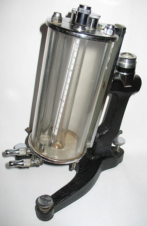
Höppler falling-ball viscometer used to determine a liquid’s viscosity from a ball’s terminal speed. The sphere accelerates briefly, then moves at constant velocity between timing marks. This instrument view adds practical context to the ball-bearing-in-liquid method discussed; minor extra details (commercial instrument hardware) are shown but are not required by the syllabus. Source
This setup provides a controlled environment for studying how drag changes with velocity.
Apparatus:
Tall transparent tube containing the viscous liquid
Micrometer or vernier caliper for measuring the ball’s diameter
Stopwatch or light-gate system for timing
Ruler or marker bands on the tube to define measurement zones
Thermometer for fluid temperature (viscosity depends on temperature)
Procedure:
Measure the radius and mass of the ball-bearing accurately.
Fill the tube with the viscous liquid and ensure no air bubbles remain.
Drop the ball-bearing into the liquid and allow it to fall.
Observe that it accelerates initially but soon reaches a constant speed.
Measure the time taken for the ball to travel between two marked points after reaching steady motion.
Repeat with several ball sizes and at constant temperature to minimise variation.
The steady speed between the markers represents the terminal velocity. Multiple trials are averaged for improved precision.
Model Cones Falling in Air
A similar method can be applied using paper cones or model parachutes falling through air. This experiment, though less precise due to air turbulence, visually demonstrates drag’s dependence on shape and surface area.
Apparatus:
Lightweight cones of known dimensions
Measuring tape and stopwatch or video analysis
Marker height from which cones are dropped
Procedure:
Release the cone from rest and observe its motion.
Record its time of fall over a measured height once it has reached steady speed.
Use video analysis or a motion sensor to plot velocity–time behaviour.
Compare results for cones of varying mass or cross-sectional area to assess how these affect terminal velocity.
This model provides an accessible illustration of drag balance in air, where the low density makes terminal velocity much higher than in liquids.
Data Analysis and Interpretation
When analysing results, plotting a velocity–time graph is essential.
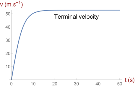
Velocity–time curve for a falling object with air resistance, approaching a constant terminal velocity. The initial steep gradient represents acceleration that decreases as drag grows, before the line becomes horizontal. The source includes parameter values and a tanh model (extra mathematical detail beyond OCR A level requirements). Source
The graph initially shows a steep gradient, representing acceleration under unbalanced forces.
The curve then levels off, showing where terminal velocity is achieved.
The horizontal section corresponds to constant speed, where weight = drag + upthrust.
By substituting measured values into Stokes’ Law, students can calculate the viscosity (η) of the fluid:
EQUATION
—-----------------------------------------------------------------
η = (2r²(ρₛ – ρₗ)g) / (9vₜ)
r = radius of sphere (m)
ρₛ = density of the sphere (kg m⁻³)
ρₗ = density of the liquid (kg m⁻³)
g = acceleration due to gravity (9.81 m s⁻²)
vₜ = terminal velocity (m s⁻¹)
—-----------------------------------------------------------------
The equation assumes laminar flow, a spherical shape, and negligible wall effects from the container. These assumptions should be considered in the evaluation of results.
Controlling Variables and Ensuring Accuracy
Accurate measurement requires control of external factors that influence drag and viscosity.
Key considerations:
Temperature control: Viscosity decreases with temperature; use a thermometer and maintain constant conditions.
Size consistency: Use identical ball-bearings to prevent drag variation due to surface imperfections.
Sufficient fluid depth: Ensure the ball achieves terminal velocity before reaching the bottom.
Elimination of air bubbles: Bubbles affect both buoyancy and flow conditions.
Repetition: Perform several trials and calculate mean terminal velocity to reduce random error.
Common uncertainties arise from timing inaccuracies, visual parallax, and non-laminar flow if the object moves too quickly. Modern data logging tools such as light gates or motion sensors improve precision significantly.
Evaluating and Extending the Experiment
Beyond simply determining terminal velocity, this investigation provides opportunities to explore:
How radius, mass, and fluid viscosity influence terminal velocity.
The transition from laminar to turbulent flow regimes at higher Reynolds numbers.
Comparison between experimental and theoretical predictions to test Stokes’ Law validity.
EQUATION
—-----------------------------------------------------------------
Reynolds Number (Re) = (ρ v d) / η
ρ = density of fluid (kg m⁻³)
v = velocity of object (m s⁻¹)
d = diameter of object (m)
η = viscosity of fluid (Pa·s)
—-----------------------------------------------------------------
When Re < 1, flow remains laminar, ensuring Stokes’ Law applies. Higher values indicate turbulence, invalidating the assumptions and producing measurement errors.
By methodically determining terminal velocity, students gain practical experience of how forces, motion, and fluid properties interrelate, reinforcing their theoretical understanding of motion with non-uniform acceleration in real-world contexts.
Practice Questions
Question 1 (2 marks)
A small steel ball is dropped into a tube of viscous liquid. After a short time, it falls at a constant speed.
(a) Explain why the ball eventually falls at a constant speed.
Mark Scheme:
1 mark: States that as the ball falls, drag (resistive force) increases with speed.
1 mark: States that terminal velocity is reached when drag (and upthrust) balance the weight so that resultant force is zero and acceleration stops.
Question 2 (5 marks)
A student determines the terminal velocity of small spheres falling through glycerol. The student measures the time taken for each sphere to travel a measured distance once it reaches constant speed.
(a) Describe how the student could ensure that the spheres have reached terminal velocity before timing their motion. (2 marks)
(b) Explain how the student could use their measurements to calculate the viscosity of the glycerol. (3 marks)
Mark Scheme:
(a)
1 mark: States that the student should allow the sphere to fall some distance before the measurement zone to ensure constant speed is reached.
1 mark: Mentions observing that the speed (or time between markers) remains constant over repeated sections of the tube.
(b)
1 mark: States that at terminal velocity, weight = upthrust + drag.
1 mark: Refers to using Stokes’ Law (F = 6πrηv) to relate drag force to viscosity.
1 mark: Explains that the viscosity η can be calculated using measured terminal velocity (v), known sphere radius (r), and densities of the sphere and fluid in the equation
η = (2r²(ρs – ρl)g) / (9v).
FAQ
Air has a much lower density and viscosity than liquids, which means resistive forces are weaker for the same velocity.
As a result, objects accelerate for longer before drag grows large enough to balance weight. However, the final terminal velocity in air is often higher because drag increases less steeply with speed than in viscous fluids.
In liquids, drag builds rapidly, so objects reach terminal velocity over shorter distances and times
Light gates detect when an object passes through a beam of infrared light, recording times automatically and eliminating human reaction errors.
They can be positioned at known distances in the steady-speed region to measure the time between gates, allowing precise calculation of terminal velocity.
Using multiple gates or a motion sensor system can verify that the velocity is constant, providing strong evidence that the sphere has truly reached terminal speed before data is used.
Errors can arise from several sources, including temperature fluctuations that change the viscosity of the fluid and inaccurate timing when using stopwatches.
If the tube is too narrow, wall effects increase drag and reduce the observed terminal velocity. Air bubbles on the sphere or in the liquid can alter both buoyancy and flow patterns.
To minimise errors:
Maintain constant temperature.
Use wide tubes relative to sphere diameter.
Ensure the liquid is degassed and clear of impurities.
Use precise timing methods such as light gates or video tracking.
Stokes’ Law assumes laminar flow, meaning fluid layers slide smoothly past each other. If the sphere is large or moves too fast, turbulent flow develops, invalidating the law.
Small spheres and viscous fluids ensure the Reynolds number remains below 1, so drag is proportional to velocity rather than velocity squared.
This keeps the motion predictable and the relationship between drag, velocity, and viscosity linear, allowing accurate application of Stokes’ Law.
Temperature affects the viscosity of liquids — as temperature rises, viscosity decreases because intermolecular forces weaken, allowing the fluid to flow more easily.
Lower viscosity reduces drag, so the same sphere will reach a higher terminal velocity.
In precise experiments, temperature should be monitored and controlled, or a correction factor applied. Using a water bath to maintain constant temperature ensures reliable and comparable data.
