AP Syllabus focus:
‘Use properties of definite integrals, including that the integral of a constant times a function and the integral of a sum can be simplified using linearity.’
The linearity of definite integrals provides efficient tools for breaking apart, scaling, and reorganizing integrals so accumulated change can be computed or interpreted more easily across diverse problems.
Understanding Linearity in Context
Linearity describes how definite integrals behave when functions are added or multiplied by constants. These properties allow students to decompose complicated integrals into simpler pieces without changing the overall value of the integral. Because definite integrals measure accumulated change across an interval, being able to restructure an integral while preserving its meaning is an essential skill.
When discussing linearity, the term definite integral refers to the signed accumulation of a function over an interval.
Definite Integral: The signed accumulated change of a function over an interval , represented by .
A central idea is that accumulation behaves predictably with respect to addition and scalar multiplication, making these properties reliable across all continuous functions on closed intervals.
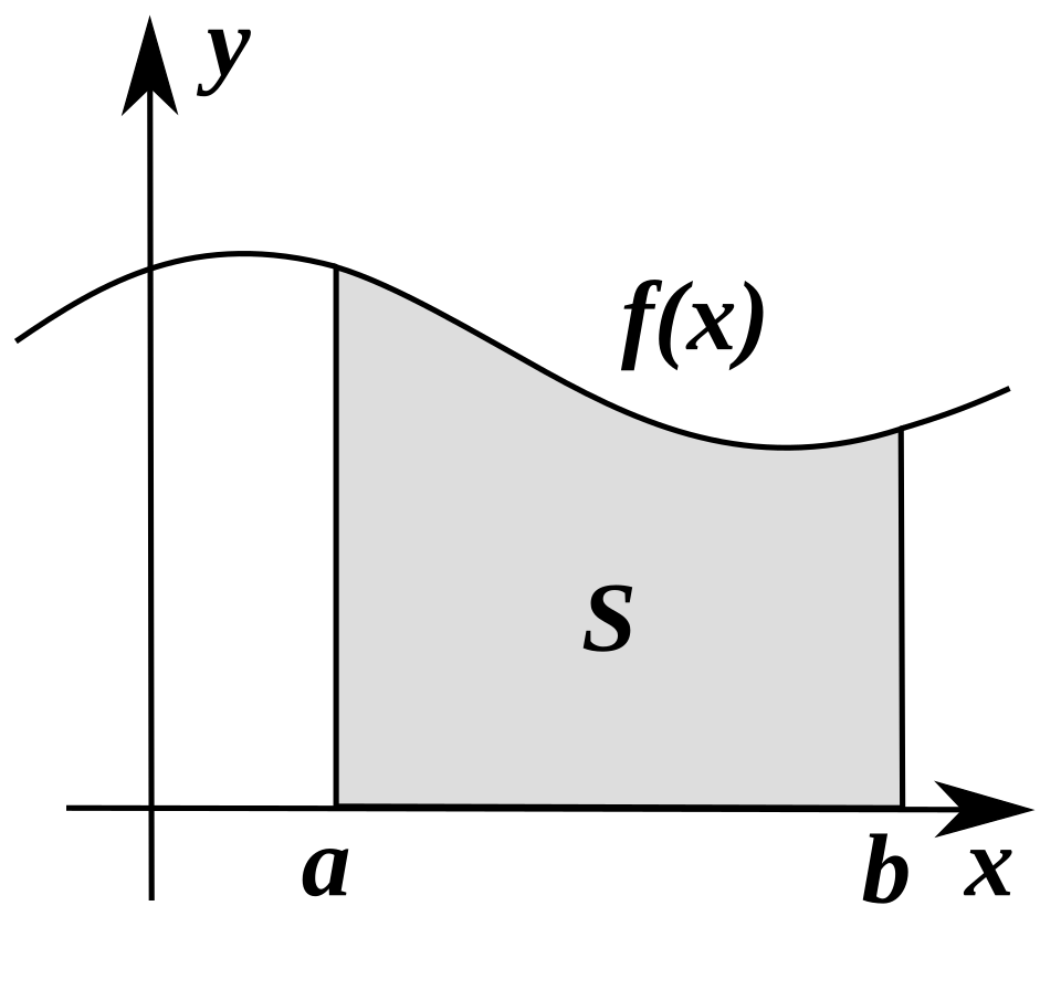
Geometrically, a definite integral represents the net signed area between the graph of a function and the x-axis over a closed interval.

A graph of a function with the region between the curve and the -axis shaded from to , representing the definite integral . The shaded region may include areas above or below the axis, illustrating that the integral measures net signed area. This supports the geometric foundation underlying linearity of definite integrals. Source.
The Additivity Property
One key component of linearity is that the integral of a sum equals the sum of the integrals. This property applies whether the functions involved represent rates, densities, or any quantities accumulated over the domain. It enables students to break a complicated integrand into manageable parts.
, = Functions representing rates or quantities accumulated over
= Bounds of integration
Because the integral is linear, accumulation distributes cleanly across addition. This property is particularly useful when an integrand consists of multiple terms with different behaviors or units.
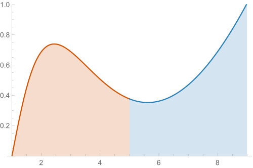
Thus, when we write , we are formally stating that the net area under the combined graph equals the sum of the net areas under the individual graphs.

A graph showing a function with shaded subregions that combine into a full interval, visually reinforcing the additive property of definite integrals. The integral over the interval is depicted as the sum of integrals over smaller pieces. The diagram includes additional structure beyond the syllabus focus, but its core message aligns with linearity. Source.
A sentence here to separate equation blocks and maintain structure.
The Constant Multiple Property
Another major component of linearity is scalar multiplication. Multiplying a function by a constant before integrating scales the total accumulated change by that same constant. This principle reinforces the idea that integrals track proportional accumulation of a quantity.
= Constant multiplier (unit depends on context)
= Function being scaled
= Bounds of integration
This property strengthens understanding of how real-world units behave. For instance, if a rate is doubled, the resulting accumulated quantity doubles as well.
Practical Uses of Linearity
Students will frequently apply linearity to rewrite integrals before calculation, estimation, or interpretation. These applications often arise in modeling contexts, such as combining different rates of change, reorganizing expressions before substitution, or identifying contributions from separate physical processes.
Reasons Linearity Is Useful
Simplifying integrands: Breaking expressions into parts that correspond to familiar antiderivative rules.
Scaling physical quantities: Understanding how multiplying a rate affects total accumulation.
Rewriting integrals for numerical methods: Making Riemann sums or trapezoidal approximations more manageable.
Connecting to units: Recognizing how constants affect rate units and, therefore, accumulated quantities.
Because linearity preserves meaning, it serves as a conceptual anchor in problems involving modeling or interpretation of accumulated change.
Distinguishing Linearity from Other Integral Properties
Linearity refers specifically to the behavior of integrals across addition and constant multiplication. It is different from, yet often used alongside, other properties of definite integrals. For example, linearity does not address how integrals behave over adjacent intervals or when reversing the order of integration limits. Those topics fall under separate rules. By maintaining this distinction, students develop a clearer sense of how each property contributes to the structure of an argument or solution.
The concept of integrable functions also matters here, since linearity requires that each function involved be integrable on the interval of interest.
Integrable Function: A function for which the definite integral over a given closed interval exists.
This ensures that each component in a linear combination contributes a well-defined amount to the accumulated change.
A sentence here provides spacing before additional structured content.
Interpreting Linearity in Real-World Terms
Because definite integrals represent accumulated change, linearity has practical meaning beyond manipulation of formulas. If two independent processes each contribute to a total accumulation, adding their rates yields a total rate whose integral is the sum of their individual accumulated amounts. Similarly, if a process occurs at a constant multiple of its original rate, accumulated change scales accordingly.
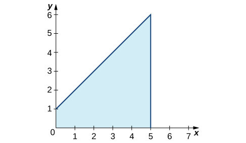
Because of linearity, we can break a complicated integrand into simpler pieces, interpret each piece as an area, and then add or scale those areas to recover the original integral.

A plot of the line with the region under the graph shaded to illustrate geometric interpretation of a definite integral. The image highlights how simple areas correspond to integrals, reinforcing the usefulness of linearity in decomposing integrands. The figure is originally used in the context of average value, which is additional content beyond this subsubtopic. Source.
Key Insights for Interpretation
Additivity reflects combined effects: If and describe separate contributions to a quantity, integrating their sum captures the total contribution.
Scalar multiplication reflects proportional processes: If a rate is increased by a factor of , the accumulation responds proportionally.
Modeling applications depend on linearity: Many composite systems rely on additive or scaled rates, which can be integrated using linear properties.
These ideas reinforce the broader conceptual theme that accumulation responds predictably to linear changes in the underlying function.
FAQ
Linearity allows you to split the definite integral across each piece of the domain, treating each segment independently before adding the results.
This is especially useful when different parts of the function behave differently or are defined using different expressions.
When combined with known geometric areas (e.g., triangles or rectangles), this greatly simplifies evaluating integrals of piecewise functions.
Yes. Differentiability is not required for linearity to hold; only integrability is needed.
A function may have corners, cusps, or other nondifferentiable behaviour and still satisfy the linearity rules as long as it remains integrable on the interval.
This makes linearity applicable to a wide range of real-world rate functions.
Scaling a function by a constant scales the accumulated quantity by the same factor.
For example:
• Doubling a rate doubles the integral’s value.
• Halving the rate halves the accumulated change.
This is helpful when interpreting unit conversions, such as converting between metres per second and kilometres per hour.
If integrals of several functions are approximated numerically (for example using Riemann sums or trapezoidal approximations), linearity guarantees that combining these approximations behaves predictably.
You can multiply approximated integrals by constants or add them together without recomputing the numerical method from scratch.
This allows greater flexibility when working with tables or discrete datasets.
Mistakes occur when students attempt to apply linearity to operations it does not govern.
Common errors include:
• Assuming the integral of a product equals the product of integrals.
• Attempting to distribute integrals over compositions such as f(g(x)).
• Treating variable-dependent coefficients as constants.
Recognising when linearity does and does not apply helps avoid invalid simplifications.
Practice Questions
Question 1 (1–3 marks)
A function h is continuous on the interval [2, 6]. It is known that
∫ from 2 to 6 of (3h(x) + 5) dx = 42.
Using the linearity of definite integrals, find the value of
∫ from 2 to 6 of 3h(x) dx.
Give a reason for your answer.
Question 1
• 1 mark: States that ∫ from 2 to 6 of 3h(x) dx = 42 − ∫ from 2 to 6 of 5 dx.
• 1 mark: Correctly evaluates ∫ from 2 to 6 of 5 dx = 20.
• 1 mark: Final answer ∫ from 2 to 6 of 3h(x) dx = 22, with a correct justification using linearity (e.g., separation of the constant term).
Question 2 (4–6 marks)
Let f and g be continuous functions on [0, 4]. The following information is known:
∫ from 0 to 4 of f(x) dx = 10
∫ from 0 to 4 of g(x) dx = -6
Consider the function p defined by
p(x) = 2f(x) - 3g(x) + 4.
(a) Use the linearity of definite integrals to write an expression for
∫ from 0 to 4 of p(x) dx
in terms of the given integrals.
(b) Hence compute the numerical value of
∫ from 0 to 4 of p(x) dx.
(c) Briefly explain why no information about the graphs of f or g is needed to answer this question.
Question 2
(a)
• 1 mark: Correctly applies linearity to produce
∫ p(x) dx = 2∫ f(x) dx − 3∫ g(x) dx + ∫ 4 dx.
• 1 mark: Identifies ∫ from 0 to 4 of 4 dx = 16.
(b)
• 1 mark: Substitutes values: 2(10) − 3(−6) + 16.
• 1 mark: Correct evaluation: 20 + 18 + 16 = 54.
(c)
• 1 mark: States that linearity relies only on integrals of the component functions, so their specific shapes or graphs are irrelevant.

