
AP Syllabus focus:
‘Apply the Intermediate Value Theorem to justify that an equation f(x) = 0 has a solution in an interval when a continuous function changes sign between the endpoints.’
Understanding how to justify the existence of a root is essential in calculus, and the Intermediate Value Theorem provides a powerful, reliable method for proving solutions must occur.
Using the Intermediate Value Theorem to Prove the Existence of a Root
The Role of Continuity in Root Existence
The Intermediate Value Theorem (IVT) applies only when a function is continuous on a closed interval. A continuous function, intuitively, has no breaks or jumps in its graph. This continuity requirement ensures that the function cannot “skip” any output values while moving from one point to another on the interval.
Continuous Function: A function with no gaps, jumps, or breaks on an interval, meaning its limit at every point equals its function value.
A normal sentence appears here to maintain required spacing before any other structured block.
When the IVT is used to justify the existence of a root, continuity guarantees that if the function starts above the x-axis and ends below it—or the reverse—it must cross the axis somewhere in between.
Statement of the Intermediate Value Theorem
The IVT states that if f is continuous on a closed interval [a, b], then the function takes on every value between f(a) and f(b) at some point in the interval. When proving the existence of a root, the value of interest is 0, because a root is a solution to the equation f(x) = 0.
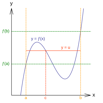
This diagram shows a continuous function on and a horizontal line at an intermediate value between and . The Intermediate Value Theorem guarantees at least one point in where . In the root-existence setting emphasized in this subsubtopic, the same picture applies with , so the horizontal line represents the x-axis and is a root. Source.
= Function values at the endpoints of the interval
= A number in the open interval where the root occurs
Why a Sign Change Implies a Root
A sign change between f(a) and f(b) indicates that the function’s outputs move from positive to negative or negative to positive. Because continuous functions cannot jump abruptly between values, the output must pass through zero in order to switch signs.
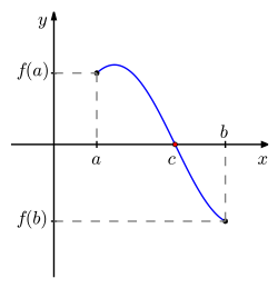
This graph illustrates a continuous function with and , so the curve must cross the x-axis at some point between and . The Intermediate Value Theorem guarantees the existence of such a point with . The specific wavy shape of the graph (a trigonometric curve) is extra detail and not essential to the IVT argument. Source.
Key ideas behind sign-change reasoning include:
Positive to negative transition implies crossing the x-axis downward.
Negative to positive transition implies crossing the x-axis upward.
Continuous motion of function values ensures no value is skipped.
Steps for Using IVT to Prove a Root Exists
Students must understand how to structure a correct IVT justification. The procedure emphasizes analytical clarity and attention to continuity.
Step-by-step reasoning
• Verify continuity on the interval: Confirm, state, or cite that the function is continuous on [a, b]. For common functions—polynomials, rational functions away from undefined points, exponentials, logarithms, and trigonometric functions—continuity follows from known properties.
• Evaluate function values at the endpoints: Compute or examine f(a) and f(b) to determine their signs.
• Check for a sign change: Ensure that f(a) · f(b) < 0, showing the function takes one positive value and one negative value.
• Apply the IVT: State that because the function is continuous and the value 0 lies between f(a) and f(b), a number c exists in the interval with f(c) = 0.
• Conclude the existence of a root: Emphasize that the IVT guarantees at least one root but does not locate it or determine how many roots exist.
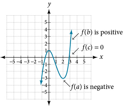
This graph of a polynomial function shows , , and a point between them where the graph crosses the x-axis. The sign change from negative to positive on a continuous graph forces at least one zero in the interval , which is exactly the Intermediate Value Theorem in action. The additional turning points of the polynomial are extra detail beyond the minimum needed for an IVT root-existence argument. Source.
Interpreting the Existence Guarantee
It is important to understand that the IVT provides existence, not the exact location of the root. Students often confuse this with solving equations numerically or algebraically, but the IVT’s purpose is entirely different: it ensures the equation f(x) = 0 has a solution without determining its value.
Distinguishing IVT from Methods of Approximation
• IVT does not give:
An explicit value of the root
The number of roots
The behavior of the function beyond the interval
• IVT does provide:A logical proof that at least one solution must exist
A foundation for numerical methods like bisection
A framework for interpreting real-world continuity-based claims
Using IVT in Contextual Situations
For real-world problems involving temperature, position, height, velocity, or other continuous quantities, the IVT supports arguments that an intermediate value—such as zero—must occur. When these contexts involve sign changes, concluding the existence of a root corresponds to asserting that the quantity becomes zero at some moment.
Logical Structure of an IVT-Based Root Argument
A strong justification always includes three essential components:
• “The function is continuous on the interval [a, b].”
• “The function values at the endpoints have opposite signs.”
• “By the IVT, there must be a number c in (a, b) such that f(c) = 0.”
These elements communicate both the required mathematical conditions and the correct application of the theorem.
Why IVT Matters in Calculus
The IVT represents one of the central ideas of calculus: continuous change implies predictable intermediate behavior. In root-existence problems, this theorem provides a rigorous bridge between sign changes and guaranteed solutions, reinforcing how calculus formalizes intuitive ideas about smoothness and continuity in mathematical and real-world settings.
Practice Questions
Question 1 (1–3 marks)
A function f is continuous on the closed interval [1, 4]. It is known that f(1) = -2 and f(4) = 5.
Use the Intermediate Value Theorem to explain why the equation f(x) = 0 has at least one solution in the interval [1, 4].
Question 1
• 1 mark for stating that f is continuous on [1, 4].
• 1 mark for identifying that f(1) and f(4) have opposite signs (negative and positive).
• 1 mark for concluding, using the Intermediate Value Theorem, that a value c in (1, 4) must exist with f(c) = 0.
Question 2 (4–6 marks)
A function g is continuous on the interval [-3, 2]. Values of g at selected points are given below:
g(-3) = 4
g(-1) = -2
g(2) = 3
(a) Show that g(x) = 0 has at least one solution in the interval [-3, -1].
(b) Explain whether the information provided is sufficient to guarantee the existence of a second root in the interval [-1, 2].
(c) State one additional condition or piece of information that would allow you to conclude there must be a second root in the interval [-1, 2].
Question 2
(a) (2 marks)
• 1 mark for stating that g is continuous on [-3, -1].
• 1 mark for noting that g(-3) = 4 and g(-1) = -2 have opposite signs, so by the Intermediate Value Theorem there must be a root in (-3, -1).
(b) (1–2 marks)
• 1 mark for stating that g(-1) = -2 and g(2) = 3 have opposite signs.
• 1 further mark for stating that continuity on [-1, 2] is required and that without explicitly confirming continuity on this subinterval, a root cannot be guaranteed.
(c) (1–2 marks)
• 1 mark for stating that confirming continuity of g on [-1, 2] would allow a conclusion about a root.
• 1 additional mark for stating that an explicit sign change at the endpoints of this interval combined with continuity would guarantee a second solution.
FAQ
The Intermediate Value Theorem guarantees that a root must occur, but it does not indicate where the root is located or how to calculate it. It is strictly an existence theorem.
To approximate a root, numerical methods such as bisection or Newton’s method are required, but these fall outside the purpose of the IVT in this subsubtopic.
No. A sign change only guarantees at least one root. The function may cross the axis multiple times between the endpoints.
To prove more than one root exists, additional information about the function’s behaviour, such as monotonicity or turning points, would be needed.
Not for that interval. A single point of discontinuity breaks the conditions required to apply the theorem.
However, the IVT may still be applied on smaller subintervals that do not include the discontinuity, provided continuity is maintained there.
The closed interval ensures both endpoint values are included, allowing you to compare f(a) and f(b) directly.
Without defined endpoint values, you cannot establish a guaranteed range of function outputs, and therefore cannot assert that the function must take on a specific intermediate value.
IVT questions often use functions where continuity is easy to justify, such as:
• Polynomials
• Basic rational functions with no discontinuities in the interval
• Trigonometric or exponential functions
These families allow students to focus on the sign-change reasoning rather than on verifying complicated continuity conditions.
