
AP Syllabus focus:
‘Develop the product rule for derivatives by applying the limit definition to a product f(x)g(x) and understanding how both factors change with x.’
The product rule emerges from examining how two varying functions interact, showing that differentiating a product requires accounting for simultaneous changes in each factor across an infinitesimally small interval.
Understanding Why a Product Needs Its Own Rule
When differentiating a product of functions, it is insufficient to treat the derivative as the product of individual derivatives. This limitation stems from the fact that both factors change simultaneously, and their combined change cannot be captured by separate differentiation alone. To justify this, AP Calculus AB emphasizes deriving the rule directly from the limit definition of the derivative, which highlights the microscopic behavior of functions as inputs shift.
Building from the Limit Definition of the Derivative
The limit definition of the derivative states that the derivative of a function at a point measures its instantaneous rate of change. For a differentiable function , this instantaneous change is captured by analyzing how compares to as becomes extremely small. Applying this foundational idea to a product requires comparing the value of the product at to its value at and then examining how this difference behaves as approaches zero.
Instantaneous Rate of Change: The limit of the average rate of change of a function as the interval length approaches zero, representing the derivative at a point.
Because the derivative relies on subtle changes in output that arise from subtle changes in input, the conceptual derivation of the product rule naturally centers on tracking how combined changes in two functions produce the total change in their product.
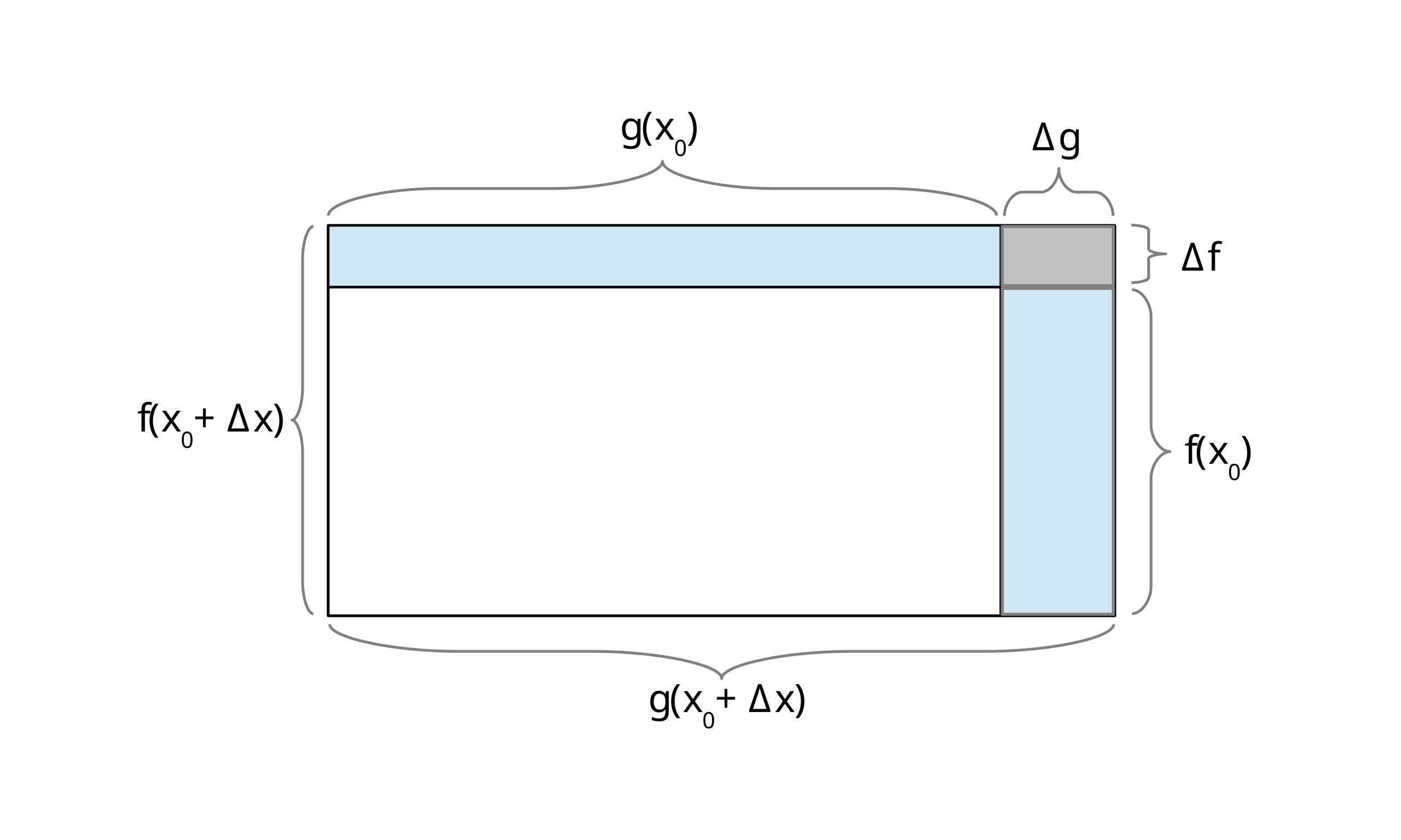
This diagram shows a rectangle whose side lengths both increase slightly, causing the total area (the product) to change. The main rectangle and its added strips visually separate the contributions from changing one factor at a time from the tiny corner term where both changes occur together. The diagram includes labels in French, which extend beyond what is strictly required but still reinforce the same geometric decomposition described in the text. Source.
Expanding the Product Difference
To derive the product rule conceptually, begin by inspecting the product under the lens of the limit definition. The expression that measures how the product changes over an interval of width is . By strategically reorganizing this expression, we can isolate the contributions from each changing factor.
= Function values at a nearby input
= Function values at the original input
After expanding and rearranging terms, a clearer picture emerges: the total change in the product comes from two sources—change in the first function while the second remains near its original value, and change in the second function while the first remains near its original value. This layered change structure is the conceptual heart of the product rule.
A key observation is that no factor remains completely unchanged, but one can treat a factor as approximately constant over extremely small intervals, which allows the limit process to isolate each contribution cleanly.
Visualizing the Dual Contributions to Change
Although formal algebraic manipulation drives the derivation, it is equally important to visualize the conceptual breakdown of changes. Each part of the expanded expression contributes to the total rate of change by representing a distinct interaction between the two functions:
Change in interacts with the approximate value of .
Change in interacts with the approximate value of .
An additional very small interaction term involving changes in both and becomes negligible as approaches zero.
This final term’s insignificance is essential, as it allows the derivative to separate into two clean components without extra complication.
Why the Combined Change Leads to the Product Rule
As the limit process eliminates the negligible interaction term and isolates the two principal contributions, the derivative of the product emerges as the sum of these contributions.
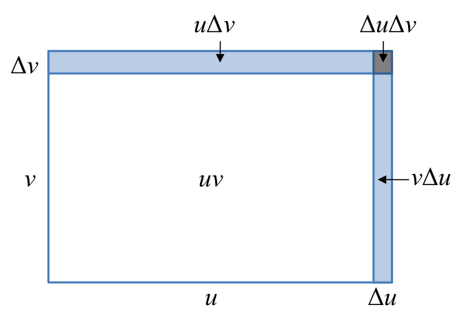
This illustration depicts a product as an area that changes when both dimensions vary slightly, with regions corresponding to the terms in the product rule. It emphasizes the two main contributions—change in one factor while the other is held approximately constant—and the smaller interaction region. The diagram uses notation and labels that may go slightly beyond the exact wording in the notes but still focus entirely on the conceptual derivation of the product rule. Source.
The conceptual leap that AP Calculus AB students must recognize is that the derivative of a product measures how each function’s instantaneous change influences the total output, not merely how the functions behave independently.
= Instantaneous rates of change of each function
= Original function values
This formula encapsulates the idea that both functions play active roles in determining the rate at which their product changes.
Understanding why this structure is necessary reinforces the broader theme in calculus that rates of change interact in nuanced ways, especially when multiple varying quantities combine.
Conceptual Takeaways for AP Calculus AB
To internalize the conceptual derivation of the product rule, students should focus on the following guiding ideas:
Differentiation of a product demands analyzing how each factor changes, not simply multiplying derivatives.
The limit definition of the derivative provides the framework for decomposing product changes.
Rearrangement of the product difference highlights that each factor’s change contributes linearly to the total instantaneous rate.
The rule arises naturally from considering infinitesimal behavior, aligning with the fundamental philosophy of differential calculus.
These insights ensure that the product rule is learned not as a memorized formula but as a meaningful consequence of how functions behave under infinitesimal change.
Practice Questions
Question 1 (1–3 marks)
The functions f and g are differentiable at x = 2. The values of f(2), g(2), f'(2), and g'(2) are shown below:
f(2) = 5
g(2) = 3
f'(2) = -2
g'(2) = 4
Using the product rule, find the value of the derivative of the product h(x) = f(x)g(x) at x = 2.
Question 2 (6 marks total)
(a) (2 marks)
• 1 mark: Clear explanation that both functions change simultaneously, so the derivative must account for each change.
• 1 mark: Statement that the limit of the product involves extra terms that cannot be captured by multiplying derivatives alone.
(b) (2 marks)
• 2 marks: Correct derivative: H'(x) = 2k(x) + (2x + 1)k'(x).
(c) (2 marks)
• 1 mark: Correct substitution into the derived expression.
• 1 mark: Final value: H'(1) = 2(4) + (3)(-3) = 8 - 9 = -1.
Question 2 (4–6 marks)
A function H is defined by H(x) = (2x + 1)k(x), where k is differentiable for all real x.
(a) Using first principles (the limit definition of the derivative), explain why the derivative of a product of two functions cannot be found by simply multiplying their individual derivatives.
(b) Derive an expression for H'(x) using the product rule.
(c) Given that k(1) = 4 and k'(1) = -3, find the value of H'(1).
Question 2 (6 marks total)
(a) (2 marks)
• 1 mark: Clear explanation that both functions change simultaneously, so the derivative must account for each change.
• 1 mark: Statement that the limit of the product involves extra terms that cannot be captured by multiplying derivatives alone.
(b) (2 marks)
• 2 marks: Correct derivative: H'(x) = 2k(x) + (2x + 1)k'(x).
(c) (2 marks)
• 1 mark: Correct substitution into the derived expression.
• 1 mark: Final value: H'(1) = 2(4) + (3)(-3) = 8 - 9 = -1.
FAQ
The interaction term arises from the simultaneous change in both functions over an interval h. Its size is proportional to h multiplied by another small change, making it significantly smaller than the main linear terms.
As h approaches zero, this interaction term shrinks much faster than the others, becoming negligible in the limit process. This is why it does not contribute to the final derivative.
The area model is a visual analogy rather than a literal requirement. It works because changing a product mimics changing the dimensions of a rectangle, even if the original functions have nothing to do with geometry.
What matters is the structural idea:
• One function changes while the other remains approximately constant.
• Then the roles reverse.
This reasoning applies to all differentiable products, regardless of context.
Local linearity states that differentiable functions behave like straight lines over very small intervals. When two such functions are multiplied, each behaves linearly at a tiny scale.
The product rule emerges because both linear approximations interact:
• One line shifts while the other is held nearly constant.
• Then the effect of the second line’s shift is added.
This reveals why the derivative breaks into two additive parts.
Yes, but the conceptual depth is reduced. Without limits, one can interpret the rule using linear approximations: each function contributes a part to the change in the product.
However, the most rigorous understanding still comes from the limit definition, as it explains precisely why the derivative of a product is not simply the product of derivatives.
The formula appears asymmetric because it distinguishes between which function is being differentiated at each stage. In practice, the expression f'(x)g(x) + f(x)g'(x) is symmetric when viewed as a sum of two contributions.
Commutativity is preserved because the order of the terms does not affect the final value, even though the decomposition highlights separate roles for each function.
