AP Syllabus focus:
‘Describe a Riemann sum as a sum of products, each equal to a function value at a chosen point in a subinterval times the length of that subinterval.’
A Riemann sum provides a foundational numerical method for approximating accumulated change by multiplying function values with subinterval widths, revealing how integrals emerge from structured discrete products.
Understanding Riemann Sums as Sums of Products
A Riemann sum expresses an approximation of accumulated change by partitioning an interval into subintervals, selecting a point within each subinterval, evaluating the function there, and multiplying that value by the subinterval’s width. This process directly supports the syllabus requirement to describe a Riemann sum as a sum of products formed from function values and subinterval lengths.
Riemann sums are essential because they represent the bridge between discrete approximations and continuous integration. By understanding them as structured products, students can interpret definite integrals as limits of increasingly refined approximations.
Partitioning an Interval
When constructing a Riemann sum, the first step is choosing a way to divide the interval.
Partition refers to a collection of points that divide an interval into smaller pieces.
Partition: A finite set of points dividing into subintervals used to approximate an integral.
Once an interval is partitioned, each subinterval has its own width. These widths may be equal or unequal depending on the problem’s context.

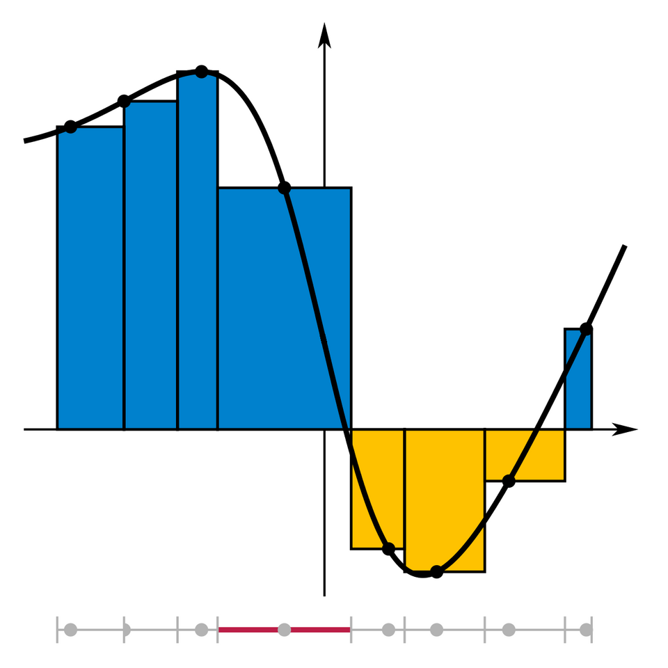
A function is shown with rectangles of varying widths and heights illustrating a general Riemann sum over nonuniform subintervals. Each rectangle’s area represents a product , and the total approximates accumulated change. The image includes additional integrand and interval details not required by the syllabus but still reinforces the core structure of Riemann sums.* Source.
After introducing a partition, it becomes possible to systematically evaluate the function at selected points that represent each subinterval.
Subinterval Widths and Sample Points
Every Riemann sum requires a choice of sample point, the location within each subinterval where the function is evaluated.
Sample Point: A chosen value within a subinterval where the function is evaluated when forming a Riemann sum.
Common choices include left endpoints, right endpoints, and midpoints, though any point inside the subinterval is acceptable. The location of the sample point influences the numerical approximation’s accuracy and relation to graph behavior.
Because sample points carry the function information, they define how the Riemann sum represents the changing quantity over the interval.
The Product Structure of Riemann Sums
At the core of this subsubtopic is the understanding that a Riemann sum is fundamentally a sum of products. Each product multiplies a function value by the width of the subinterval over which that value is assumed to represent the rate of change.
= Riemann sum approximation of accumulated change
= function value at the chosen sample point
= width of the subinterval
This equation highlights the syllabus emphasis: each term in the sum reflects a function value multiplied by a subinterval length, capturing how much the function contributes to the total over that region.
Between these structured components lies the interpretation of how discrete pieces approximate continuous accumulation.
Conceptual Interpretation of Each Product
Each product reflects an estimate of how much the quantity being modeled changes across the subinterval. The function value represents the rate, while the width represents the duration or extent over which that rate acts.
Key ideas to understand include:
Rate × duration = accumulated change, matching physical interpretations such as velocity × time = displacement.
The function value serves as an estimate of the entire subinterval’s behavior.
Smaller subintervals typically improve accuracy by reducing variation within each interval.
The sum of these products synthesizes local approximations into a global total.
The structure invites students to see integration as the natural extension of this accumulation.
Types of Riemann Sums
While this subsubtopic does not focus on specific types, it is essential to connect the concept of sums of products to the choices made when selecting sample points. Variants follow the same fundamental product structure:
Left Riemann Sum: sample points are left endpoints.

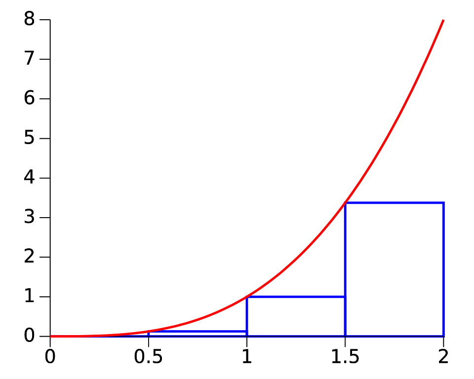
The graph depicts a left Riemann sum where rectangle heights are determined by left endpoints of equal subintervals. Each area is the product , reinforcing the structure of Riemann sums. The exact function and interval shown include more detail than required but effectively illustrate the left-endpoint idea.* Source.
Right Riemann Sum: sample points are right endpoints.
Midpoint Riemann Sum: sample points are midpoints.

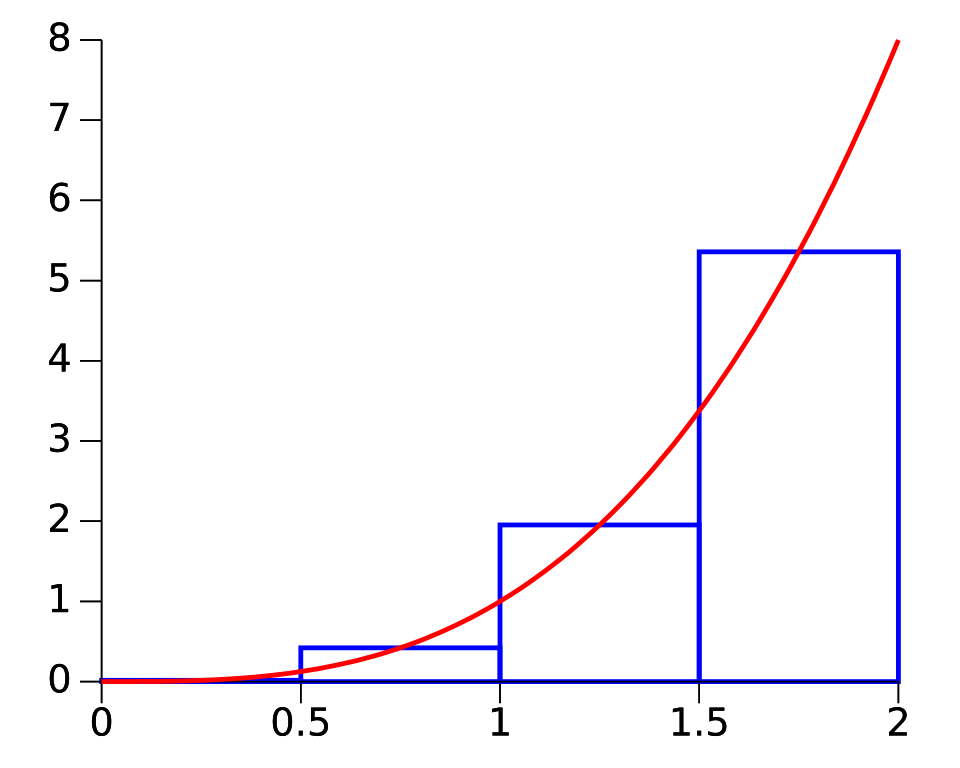
The graph shows rectangles constructed using midpoint sampling, forming a midpoint Riemann sum. Each rectangle models a product , demonstrating how different sample points still follow the same sum-of-products structure. The specific function and interval exceed syllabus needs but support conceptual clarity.* Source.
General Riemann Sum: sample points may be anywhere in each subinterval.
All of these conform to the syllabus description because each still involves products of function values and subinterval widths.
These variations demonstrate how different sampling choices affect the approximation while maintaining the same mathematical structure.
Building Toward the Definite Integral
Understanding Riemann sums as sums of products prepares students for interpreting definite integrals as limits of these sums when subinterval widths become arbitrarily small. The refinement of partitions and the accumulation of increasingly precise products lead naturally to the concept of integration.
This subsubtopic lays the groundwork for the formal definition of the definite integral and the conceptual leap from approximation to exact accumulated change in later topics.
FAQ
The accuracy depends on how well the sample point represents the function’s behaviour over the subinterval. If the function is increasing, a right-endpoint sum will tend to overestimate, while a left-endpoint sum will tend to underestimate.
Midpoint sums are generally more accurate because they better capture the average behaviour of the function on each subinterval.
For highly irregular functions, decreasing the subinterval widths usually has a greater impact on accuracy than changing sample point type.
A Riemann sum does not require equal subinterval widths; it only requires that each subinterval has a defined length and a chosen sample point.
Non-uniform partitions are useful when the function changes more rapidly in certain regions, allowing narrower subintervals to better capture behaviour where needed.
As long as subinterval widths tend to zero in the limit, the resulting sum still represents the integral.
The function must be integrable on the interval, which is guaranteed if it is continuous or has only a small number of removable or jump discontinuities.
Additionally, the maximum subinterval width must approach zero as the number of subintervals increases.
Under these conditions, any Riemann sum—regardless of sampling method—converges to the same value.
Not all applications involve spatial area. A Riemann sum measures accumulated change, which may represent distance, volume, mass, or any quantity with an associated rate.
The product structure generalises the concept: rate multiplied by interval length equals change.
This framing allows Riemann sums to be applied meaningfully to contexts that have no geometric interpretation.
General Riemann sums allow sample points to be chosen strategically rather than mechanically.
This is useful when:
Certain points provide better information about functional behaviour.
Data are only available at irregularly spaced inputs.
A model requires weighting particular locations within a subinterval.
Such flexibility enables more accurate or context-appropriate approximations without altering the overall structure of the Riemann sum.
Practice Questions
(1–3 marks)
A function f is defined on the interval 2 ≤ x ≤ 6. The interval is divided into four equal subintervals, and the sample point in each subinterval is chosen to be its right endpoint.
Write an expression for the Riemann sum that approximates the accumulated change of f over the interval using this partition.
(1–3 marks)
• 1 mark: Correct expression for the width of each subinterval: 1.
• 1 mark: Correct identification of right endpoints: 3, 4, 5, 6.
• 1 mark: Correct Riemann sum expression: f(3) + f(4) + f(5) + f(6).
(Allow equivalent expressions such as a factor of 1 multiplying the sum.)
(4–6 marks)
A function g models the rate of change of a quantity. The interval 0 ≤ x ≤ 3 is divided into three subintervals: [0, 1], [1, 1.5], and [1.5, 3]. Sample points are chosen to be 0.5, 1.25, and 2 respectively. The corresponding function values are g(0.5) = 4, g(1.25) = 6, and g(2) = 3.
(a) Construct the Riemann sum that approximates the total accumulated change of the quantity over the interval.
(b) Explain in words what each term of your sum represents in the context of accumulation.
(c) State how the approximation would generally change if more subintervals of smaller width were used.
(4–6 marks)
(a)
• 1 mark: Correct widths: 1, 0.5, and 1.5.
• 1 mark: Correct Riemann sum: 4(1) + 6(0.5) + 3(1.5).
(b)
• 1 mark: States that each term represents the estimated change on the corresponding subinterval.
• 1 mark: Identifies that the function value gives the rate and the subinterval width gives the duration/extent.
(c)
• 1 mark: States that using more, smaller subintervals generally increases accuracy.
• 1 mark: States that the approximation would more closely reflect the true accumulated change (integral).

