
AP Syllabus focus:
‘Instructions on how to use residual plots to describe the form of association of bivariate data, specifically looking for evidence of linearity. It will elaborate on how the apparent randomness or lack thereof in a residual plot can indicate the adequacy of a linear model for the data set, thereby guiding decisions about model suitability.’
Residual plots play a central role in evaluating whether a linear model appropriately represents a relationship between two quantitative variables, helping reveal structure hidden in the original scatterplot.
Interpreting Residual Plots for Linearity
Residual plots are essential diagnostic tools in regression analysis because they help determine whether a linear model is suitable for a given data set. A residual is defined as the difference between an observed value and its predicted value from a regression model. Residual plots graph these residuals against either the explanatory variable or the predicted values to assess whether a linear pattern is appropriate. According to the AP Statistics specification, students must be able to identify whether a residual plot shows apparent randomness, which would support a linear model, or systematic patterns, which suggest that the linear model is inadequate.
What Residual Plots Reveal About Linearity
Residual plots help uncover structure that might not be apparent in the original scatterplot. When a linear model is appropriate, the residuals should display no identifiable pattern. Instead, they should be randomly scattered around zero, indicating that the linear model captures the trend without missing important curvature or systematic behavior. The goal is to determine whether the relationship between the variables is truly linear or whether another model would provide a better representation.
Understanding Key Terminology in Residual Plot Interpretation
When evaluating residual plots, several important terms guide the analysis. The explanatory variable is the variable used to predict the response variable in a regression model. The response variable is the variable being predicted. Residual plots provide insight into how well the chosen model captures this predictive relationship.
Residual: The difference between an observed value of the response variable and the corresponding predicted value from the regression model ().
Residuals measure prediction error. When these errors are plotted, their arrangement helps analysts judge whether the model assumptions hold.
Characteristics of a Residual Plot Supporting Linearity
A residual plot that supports linearity should reflect:
Random scatter around zero, with no visible pattern.
Uniform spread, indicating consistent variability across the range of x-values.
Absence of curves, waves, clusters, or directional trends.
Minimal outliers, as extreme residuals may suggest an issue with the model.
These features signal that the linear model is capturing the underlying trend and that no additional structure—such as curvature—needs to be modeled.
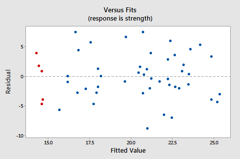
Residuals appear randomly scattered around zero with roughly constant variability, illustrating the conditions under which a linear model is considered appropriate. Source.
Indicators That a Linear Model Is Inappropriate
A residual plot that shows non-random structure implies that a linear model does not appropriately describe the relationship. Students should be able to recognize several common patterns that indicate model inadequacy:
Curvature, such as a U-shape or inverted U-shshape, suggesting a nonlinear relationship.
Funnel shapes, where the spread increases or decreases across x-values, indicating non-constant variability.
Clusters, which may suggest subgroups or omitted variables.
Systematic positive or negative sequences, showing that the model consistently overpredicts or underpredicts in certain regions.
Such features imply that the linear assumptions of constant variance and model form are violated.
This residual plot displays a distinct U-shaped pattern, demonstrating a violation of linearity because the model systematically mispredicts across different regions of the explanatory variable. Source.
Why Apparent Randomness Matters
Residual plots aim to show whether model errors behave as expected under linear regression assumptions. Apparent randomness demonstrates that the model does not leave behind unexplained structure. In contrast, lack of randomness signals that the model misses some underlying behavior. The AP specification emphasizes that students must carefully observe residual plots because even a strong correlation or well-fitting line on a scatterplot does not guarantee the appropriateness of a linear form.
Steps for Interpreting a Residual Plot
Students analyzing residual plots for linearity should follow a set of structured steps:
Locate the horizontal axis at residual = 0 and observe how points scatter above and below it.
Check for noticeable patterns, such as curves or clusters.
Evaluate the spread to determine whether variability appears constant across x-values.
Identify potential outliers, which may disproportionately influence the regression model.
Decide whether the residual plot supports a linear model, based on the presence or absence of structure.
Following these steps ensures consistency and accuracy.
How Residual Plots Guide Modeling Decisions
Residual plots help determine whether to retain the linear model or explore alternatives. A plot exhibiting randomness suggests that linear regression is appropriate. A plot showing non-random features may lead analysts to consider nonlinear models or transformations. The AP syllabus highlights that evaluating the form of association using residual plots is a critical part of assessing overall model suitability, ensuring that regression analysis accurately reflects the data’s behavior.
Strengthening Interpretation Skills
Developing proficiency in interpreting residual plots allows students to move beyond surface-level observations. Understanding how residuals reveal structural issues equips learners to make informed judgments about the appropriateness of a model. Since residual plots show what the regression model fails to explain, they serve as powerful tools for assessing linearity in accordance with AP Statistics expectations.
FAQ
Residual plots from small samples may look more irregular simply because each observation has a larger influence. Apparent patterns can emerge by chance even if the underlying relationship is linear.
With larger samples, random variation tends to balance out, making true structural patterns easier to detect. This is why stronger conclusions about linearity usually rely on moderate to large data sets.
Yes. In some cases, a curved scatterplot may visually exaggerate patterns due to changes in scale or the presence of influential points.
A well-constructed residual plot removes the linear trend, making structure easier to spot. If residuals still appear random after removing that trend, the underlying relationship may actually be close enough to linear for modelling purposes.
Measurement error in either variable increases the scatter of residuals, making patterns harder to detect. This can mask curvature or other structural issues.
If measurement errors are systematic rather than random, they may create misleading patterns in the residual plot, such as directional bias or irregular clustering.
Plotting residuals against x is often preferred when checking linearity, as it directly shows how errors vary across the explanatory variable.
Plotting residuals against predicted values can highlight issues related to the fitted model rather than the original variable scale. Both approaches can be useful, but each emphasises slightly different sources of structure.
Yes. When residuals form clusters or show different behaviours across groups of observations, this may suggest that an omitted variable influences the response.
Signs that another variable might be needed include:
• distinct bands of residuals
• consistent overprediction or underprediction for particular subgroups
• changing variability associated with identifiable conditions
Practice Questions
Question 1 (1–3 marks)
A researcher fits a linear regression model to a set of bivariate data and creates a residual plot. The residuals appear randomly scattered around zero with no visible pattern.
a) Based on the residual plot, explain whether a linear model is appropriate.
b) Give one reason why residual plots are useful when evaluating regression models.
Question 1
a)
• 1 mark: States that the linear model is appropriate.
• 1 mark: Justifies based on random scatter around zero and absence of patterns.
(Max 2 marks)
b)
• 1 mark: States that residual plots help assess whether the model captures the form of the relationship (e.g., identify nonlinearity, detect patterns, evaluate model fit).
(Max 1 mark)
Question 2 (4–6 marks)
A student analyses the relationship between two quantitative variables: study time (hours) and test score (points). After fitting a linear regression model, the student produces a residual plot. The plot shows that residuals are mostly negative at low study times, mostly positive at moderate study times, and negative again at high study times.
a) Describe the pattern in the residual plot.
b) Explain what this pattern indicates about the suitability of the linear model.
c) Suggest one action the student might take to improve the modelling of the relationship, justifying your suggestion.
Question 2
a)
• 1 mark: Correctly identifies a curved or systematic pattern (e.g., U-shaped).
• 1 mark: Clearly describes how residuals change across the range (negative–positive–negative).
(Max 2 marks)
b)
• 1 mark: States that the pattern indicates the relationship is not linear.
• 1 mark: Explains that the model systematically overpredicts and underpredicts in different regions, violating linearity assumptions.
(Max 2 marks)
c)
• 1 mark: Suggests an appropriate action (e.g., consider a nonlinear model, apply a transformation, examine polynomial regression).
• 1 mark: Provides a clear justification linking the action to correcting the curvature or improving model fit.
