
AP Syllabus focus:
‘Determine when it is appropriate to use the normal distribution to approximate probabilities for unknown distributions. Normal distributions, being symmetrical and bell-shaped, can approximate distributions with similar characteristics effectively. This concept involves evaluating the shape and characteristics of a given distribution to decide if the normal distribution is a suitable model for approximation.’
The normal distribution is frequently used in statistics, but it is essential to determine when this approximation is appropriate, especially when the underlying population distribution is unknown.
Evaluating When Normal Approximation Is Reasonable
Understanding when to use a normal distribution requires assessing the characteristics of the underlying data or distribution. A normal distribution is symmetrical, unimodal, and bell-shaped, and these attributes guide when a normal approximation produces accurate probability estimates. When the true population distribution is unknown, these observable features from a sample help determine suitability.
Key Characteristics of a Normal Distribution
The normal distribution is defined by its familiar bell-shaped curve and symmetry around the mean.
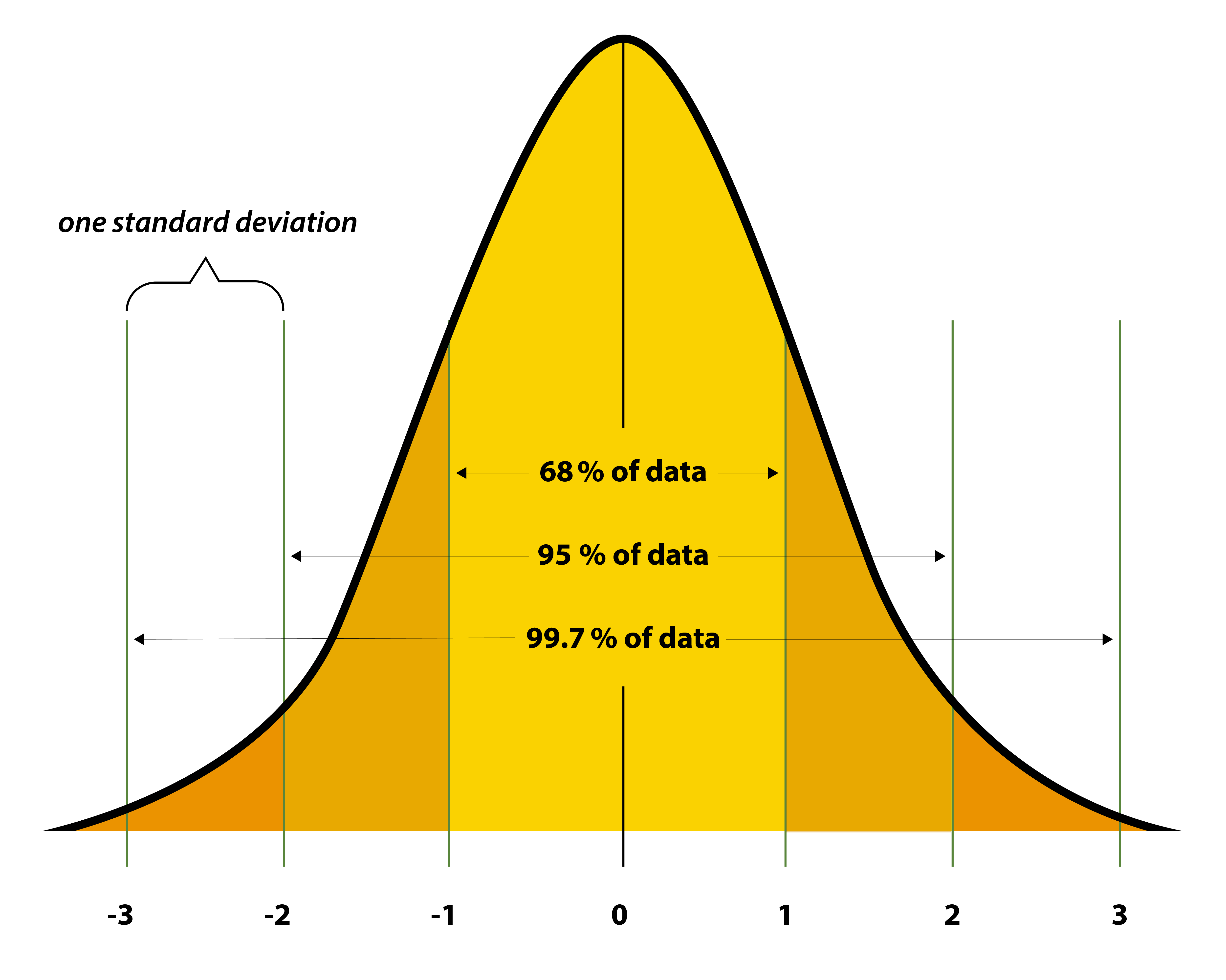
Standard normal distribution curve illustrating symmetry, a single central peak, and decreasing tail probabilities. The shaded percentage regions extend slightly beyond the syllabus by showing the empirical rule but help reinforce how area represents probability. Source.
These traits make it a powerful model for approximating probabilities, particularly because many natural and social processes produce distributions resembling or converging toward normality through repeated, independent contributions from numerous small influences.
Normal Distribution: A continuous, symmetrical, bell-shaped probability distribution defined by its mean and standard deviation.
When evaluating data, confirming whether these characteristics are present supports choosing the normal model as an approximation for probability calculations.
Assessing Shape When the Population Distribution Is Unknown
Because the syllabus emphasizes working with situations in which the underlying distribution is unknown, students must rely on sample-based evidence to judge appropriateness. This involves observing patterns in sample histograms, dotplots, or stem-and-leaf distributions to determine resemblance to a normal curve.
Visual and Descriptive Indicators of Approximate Normality
Students use both visual and descriptive tools to check for normal-like behavior. Each tool provides insight into different aspects of distribution shape.
Symmetry
A roughly centered peak with evenly balanced tails suggests normal-like behavior.
Significant skewness indicates that the normal approximation may not be appropriate.
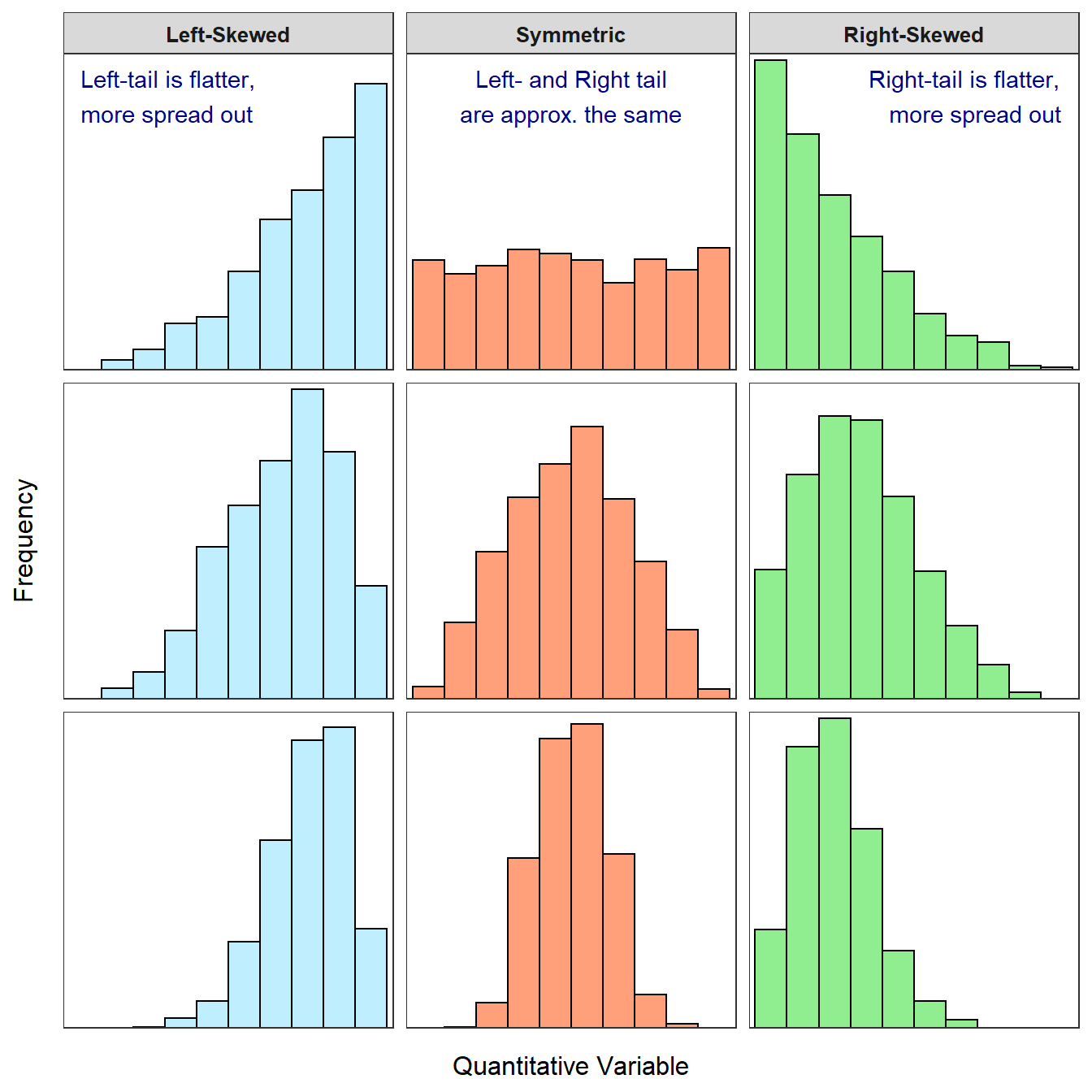
Histograms illustrating varying degrees of left skewness, symmetry, and right skewness. The symmetric shapes align well with normal approximation, while skewed shapes demonstrate when the approximation becomes unreliable. Source.
Unimodality
A single, prominent peak supports a normal approximation.
Multiple peaks suggest heterogeneity or subpopulations that violate normal assumptions.
Tail behavior
Tails that decrease smoothly and gradually resemble normal curves more closely.
Heavy-tailed or extremely light-tailed shapes deviate from normality.
Normal approximations rely on these features being present to a reasonable degree, even if not perfectly.
When Normal Approximation Is Most Effective
The normal distribution is particularly effective in approximating unknown distributions under conditions where randomness accumulates and individual deviations are small. This aligns with many real-world scenarios in which outcomes arise from additive processes.
Situations Favoring Normal Approximation
Certain contextual factors make normal approximation more trustworthy:
The variable represents aggregated or averaged outcomes from many small influences.
The distribution exhibits no extreme outliers or sharp discontinuities.
Sample size is reasonably large, making irregularities less impactful.
Although the Central Limit Theorem applies specifically to sample means, the general idea that larger samples stabilize irregularities helps justify normal approximation for other contexts as well.
A normal sentence between definition blocks improves readability.
Skewness: A measure of the asymmetry of a distribution, indicating whether data values tail more heavily to the left or right.
Judging Appropriateness Using Context and Purpose
Determining suitability is not solely about visual resemblance; it also depends on how the normal distribution will be used for probability approximation. Even if a distribution is imperfectly normal, the approximation may still yield useful results if the degree of deviation is small relative to the required precision.
Contextual Considerations
Students should consider the purpose and stakes of the probability estimate:
High-stakes decisions require stronger evidence of normality.
Exploratory analysis or approximate reasoning can tolerate mild deviations.
Practical constraints may favor a normal approximation when computational tools for the exact distribution are unavailable.
Because the normal distribution simplifies probability computation, especially through z-scores and standardization, it remains the preferred model when conditions do not severely violate normal-like behavior.
Limitations and Restrictions of Normal Approximation
Despite its usefulness, the normal approximation should not be applied indiscriminately. Some distributions inherently contradict the assumptions of normality.
Situations Where Normal Approximation Is Not Appropriate
A normal model should be avoided when:
The distribution is highly skewed or heavily tailed.
Data include structural boundaries, such as minimum or maximum possible values, that truncate the shape.
Categorical or discrete variables do not meaningfully approximate continuous data.
Outliers or data clusters introduce non-normal patterns.
These violations compromise the symmetry and tails required for normal-like behavior, weakening probability accuracy.
Integrating Evidence From Graphical and Numerical Measures
Students must synthesize various indicators rather than relying on a single test. Observing alignment between visual tools and numerical summaries strengthens the rationale for using the normal distribution.
Combined Diagnostic Approaches
Useful approaches include:
Checking if mean and median are close, supporting symmetry.
Inspecting whether most data follow a smooth, single-peaked pattern.
Using standardized units to test for extreme departures from expectations.
Comparing sample plots to a theoretical normal curve or distribution overlay.
When these signals align, applying the normal distribution to approximate probabilities becomes reasonable and statistically justified under the syllabus guidance.
FAQ
Mild skewness does not automatically rule out a normal approximation. What matters is whether the skewness meaningfully affects the tail behaviour relevant to the probability being calculated.
If the region of interest lies near the centre of the distribution, a small amount of skew may not significantly distort results.
However, probabilities involving the extremes of the distribution are more sensitive, and even modest skewness can reduce the accuracy of a normal approximation.
Normal distributions assume a single, central peak. If a distribution has two or more peaks, each peak represents a different sub-group or process.
Using a normal approximation in such cases can mask meaningful structure, misrepresent variability, and distort probability estimates.
A unimodal shape ensures that the data behave as if generated by one underlying process, making the normal model a more reliable approximation.
Outliers can disproportionately stretch the tails of a distribution, breaking the gradual decline expected in a normal curve.
This matters because normal approximations rely on predictable tail behaviour; unusual extremes introduce abrupt tail changes that normal models cannot represent.
Before applying a normal approximation, it is advisable to investigate whether outliers reflect genuine variability or measurement error.
A larger sample provides a clearer picture of the distribution’s true shape.
With small samples, irregularities may appear that disappear with more data, making it harder to judge suitability.
Larger samples smooth out random fluctuations, enabling more confident assessments of symmetry, tail behaviour, and unimodality.
Sometimes. Slightly heavier tails may still permit normal approximation for central-area probabilities.
However, probabilities involving extreme values become less reliable because heavier tails imply more frequent extreme observations than a normal model predicts.
In practice, the normal approximation can still be used with caution, but extra attention should be given to the specific probability region being estimated.
Practice Questions
Question 1 (1–3 marks)
A researcher collects a large sample of daily temperatures from a coastal city. A histogram of the data shows a single peak and appears roughly symmetrical with no extreme outliers.
Explain whether it would be appropriate to use a normal distribution to approximate probabilities for this dataset.
Question 1
• 1 mark for identifying that the distribution is approximately symmetrical and unimodal.
• 1 mark for recognising that lack of outliers supports normal approximation.
• 1 mark for concluding that using a normal distribution is appropriate, with a brief justification based on shape.
Question 2 (4–6 marks)
A company records the waiting times (in minutes) for customers at a service desk. A preliminary analysis shows the following:
• The histogram of waiting times is moderately right-skewed.
• The mean is noticeably greater than the median.
• The distribution includes several unusually long waiting times.
(a) Discuss whether a normal distribution would be suitable for approximating probabilities based on these waiting times.
(b) Explain how the shape and features of this distribution affect the use of the normal model in practice.
(c) Suggest one modification or alternative approach the company could use if a normal approximation is not appropriate.
Question 2
(a)
• 1 mark for identifying the right skewness.
• 1 mark for recognising that skewness makes the normal distribution inappropriate.
(b)
• 1 mark for noting that the mean being greater than the median indicates asymmetry.
• 1 mark for identifying that extreme values distort tail behaviour, making the normal model unsuitable.
(c)
• 1 mark for suggesting a reasonable alternative (e.g., data transformation, using a non-parametric method, or applying a distribution better suited to skewed data).
• 1 mark for explaining why this alternative would work better than a normal approximation.
