
AP Syllabus focus:
‘The confidence interval for the difference between two population means is given by: (x̄1 - x̄2) ± (t* × SE), where x̄1 and x̄2 are the sample means, t* is the critical value from the t-distribution, and SE is the standard error of the difference. The critical t-values are chosen based on the desired confidence level and degrees of freedom, which can be determined using technology such as a calculator or statistical software. The degrees of freedom can be estimated using a formula that accounts for the sample variances and sizes, which is also provided by many statistical software packages.’
Constructing a confidence interval for the difference of two means allows researchers to estimate how two populations compare while acknowledging sampling variability and uncertainty in real data.
Calculating a Confidence Interval for the Difference of Two Means
A confidence interval for the difference between two population means quantifies plausible values for μ₁ − μ₂, helping determine whether the means differ in a meaningful way. This process applies when two samples are independent and the goal is to estimate the difference of their associated population means.
Understanding the Interval Structure
A confidence interval for the difference of means is built around the point estimate—the observed difference in sample means, x̄₁ − x̄₂. This estimate reflects the best available single-value approximation for the population difference. However, because sample data vary, the point estimate alone is insufficient for inference, requiring the incorporation of a margin of error to express uncertainty.
When the population standard deviations are unknown, the t-distribution becomes the foundation of inference. The t-distribution adjusts for the additional variability introduced by estimating standard deviations from sample data. Its shape depends on degrees of freedom, which influence how wide the interval becomes.
Required Components for the Interval
To calculate the interval, three components are essential: the point estimate, the critical value, and the standard error of the difference. Each one contributes to the accuracy and interpretability of the interval.
Point Estimate: The observed difference between sample means, x̄₁ − x̄₂, serving as the best estimate of μ₁ − μ₂.
The confidence interval expands outward from the point estimate according to the magnitude of its standard error and the desired confidence level. Higher confidence levels require wider intervals because they use larger critical values from the t-distribution.
The Standard Error of the Difference
The standard error measures how much the sample mean difference is expected to vary from sample to sample.
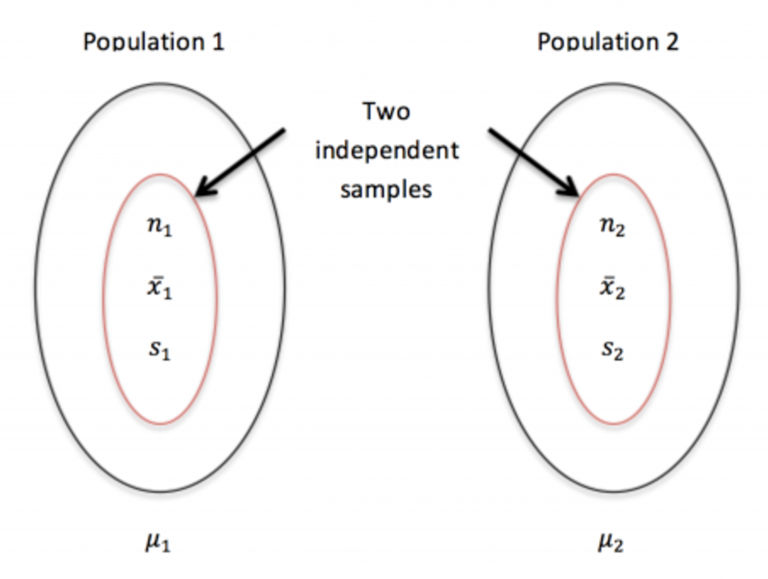
This diagram shows two independent populations, each with its own sample size, sample mean, and sample standard deviation. The notation matches the quantities used in the standard error formula for the difference of two means. It reinforces that variability in the difference of sample means depends on both samples. Source.
EQUATION
= Sample standard deviations for groups 1 and 2
= Sample sizes for groups 1 and 2
This expression shows that greater sample variability increases the standard error, while larger sample sizes reduce it. The interval thus reflects the combined precision of both samples.
A normal sentence is placed here to separate equation blocks, ensuring clarity and readability.
The Role of the Critical Value
The critical value, denoted t*, determines how far the interval extends from the point estimate for a given confidence level. It comes from the t-distribution with degrees of freedom determined either through statistical software or through an approximation method. As required by the syllabus, technology may be used to compute this value precisely, particularly because the degrees of freedom for two-sample procedures involve a more complex formula.
Critical Value (t*): A cutoff from the t-distribution that reflects the chosen confidence level and degrees of freedom, determining the width of the margin of error.
Degrees of freedom influence the shape of the t-distribution, especially when sample sizes are small.
This plot shows a t-distribution with shaded areas marking the rejection regions for a two-sided test at α = 0.05. The central region corresponds to the middle probability that defines the confidence level. Although often used in hypothesis testing, these same critical values determine the width of t-based confidence intervals. Source.
Constructing the Confidence Interval
After computing the standard error and identifying the appropriate critical value, the confidence interval for the difference of means is assembled using a standard structure. The syllabus specifies the required form, which centers the interval at the point estimate and extends it by the product of t* and the standard error.
EQUATION
= Sample means of groups 1 and 2
= Critical t-value for the selected confidence level
= Standard error of the difference between sample means
This interval captures a range of plausible values for μ₁ − μ₂, indicating whether the population means may differ and by how much. If the interval contains zero, it suggests that no difference in means is consistent with the sample data. If zero lies outside the interval, the data support the existence of a meaningful difference.
Interpretation Considerations
Interpreting the resulting interval must always occur within the context of the populations being compared. Students should recognize that the procedure relies on independent samples, approximate normality of sampling distributions, and appropriate degrees of freedom. The computed interval conveys uncertainty but not causation; it describes the strength and precision of evidence regarding the difference in population means.
FAQ
When sample sizes differ substantially, the standard error becomes more influenced by the group with the smaller sample size because it contributes more variability.
This can widen the confidence interval, reducing precision.
Researchers often aim for reasonably balanced sample sizes to achieve a more stable estimate of the difference between population means.
Yes, but only if both samples also have large sample sizes.
A large n reduces each variance term in the standard error calculation, offsetting the effect of high variability.
However, if sample sizes are small, large standard deviations nearly always lead to a wide interval.
Some statistical software uses a more exact method for calculating degrees of freedom, rather than relying on a simplified approximation.
This method can yield slightly different upper and lower bounds, creating an interval that is not perfectly symmetric around the point estimate.
The asymmetry reflects adjustments for unequal variances and sample sizes.
The procedure is highly sensitive because the formula assumes no relationship between the samples.
If the samples are dependent, the calculated standard error will be incorrect, often leading to an interval that falsely appears more precise.
In such cases, a paired analysis is required instead.
If the standard error is already very small—typically due to large, well-behaved samples—increasing the confidence level may widen the interval only modestly.
In these situations, the t-distribution’s critical values flatten out, so the difference between levels such as 90% and 95% becomes less dramatic.
Practice Questions
Question 1 (1–3 marks)
A researcher compares the mean reaction time of two independent groups: participants who consumed caffeine (Group 1) and participants who did not (Group 2).
The sample means are 242 ms for Group 1 and 257 ms for Group 2.
A 95% confidence interval for the difference in population means (Group 1 minus Group 2) is calculated to be:
-22 ms to -8 ms.
(a) Based on this interval, what does the result suggest about the mean reaction times of the two populations?
(b) Briefly explain why this interval supports your conclusion.
Question 1
(a)
• 1 mark: States that the population mean reaction time for the caffeine group is likely lower than that of the non-caffeine group.
(b)
• 1 mark: Explains that the entire confidence interval is below zero, indicating a consistent negative difference (Group 1 minus Group 2).
• 1 mark: Recognises that because zero is not included, the data suggest a genuine difference in population means.
Question 2 (4–6 marks)
Two independent random samples are taken to compare average waiting times at two hospital departments.
Sample 1 (Department A): n1 = 40, mean = 27.4 minutes, standard deviation = 6.1 minutes
Sample 2 (Department B): n2 = 35, mean = 31.8 minutes, standard deviation = 7.5 minutes
A 90% confidence interval for the difference in population means (A minus B) is calculated as:
-6.9 minutes to -1.9 minutes.
(a) Interpret this confidence interval in context.
(b) State what the interval suggests about the relative waiting times of the two departments.
(c) Explain why the t-distribution is appropriate for this confidence interval.
Question 2
(a)
• 1 mark: States that the interval suggests the true difference in mean waiting times (A minus B) lies between -6.9 and -1.9 minutes.
• 1 mark: Interprets that Department A’s mean waiting time is estimated to be between about 2 and 7 minutes shorter than Department B’s.
(b)
• 1 mark: Clearly states that Department A appears to have a shorter average waiting time because the entire interval is negative.
• 1 mark: Notes that zero is not included, indicating a meaningful difference between the departments’ population means.
(c)
• 1 mark: Points out that population standard deviations are unknown, so sample standard deviations must be used.
• 1 mark: States that this requires the t-distribution for inference, especially with moderately sized samples.
