
AP Syllabus focus:
‘When comparing two means from independent random samples with each population modeled normally, the test statistic is calculated using the formula: t = (x̄1 - x̄2 - (μ1 - μ2)) / √(s1²/n1 + s2²/n2), where x̄1 and x̄2 are sample means, μ1 and μ2 are population means (often μ1 - μ2 = 0 under H0), s1 and s2 are sample standard deviations, and n1 and n2 are sample sizes. - Degrees of freedom for this t-test are estimated using technology, falling between min(n1-1, n2-1) and (n1 + n2 - 2).’
Understanding how to calculate the test statistic in a two-sample t-test for the difference of means is essential because it quantifies how far the observed difference deviates from the hypothesized difference.
Calculating the Test Statistic for Two Population Means
The goal of the two-sample t-test is to compare the means of two independent populations when the population standard deviations are unknown. The test statistic provides standardized evidence about whether an observed difference in sample means is consistent with the hypothesized difference in the population means.
The Structure of a Two-Sample t-Statistic
The test statistic measures how many standard errors the observed sample difference lies from the hypothesized difference. Because the true population standard deviations are unknown, the calculation requires sample statistics and an estimate of variability. This aligns with the syllabus requirement that the statistic follows a t-distribution when sample standard deviations replace population values.
EQUATION
= Test statistic describing standardized difference
= Sample means from populations 1 and 2
= Hypothesized population mean difference
= Sample standard deviations
= Sample sizes
Because this formula relies on the standard error of the difference in sample means, it directly incorporates both the variability and the sizes of the two independent samples.
Understanding the Components of the Test Statistic
Each part of the formula carries a distinct conceptual meaning that governs how the test statistic behaves.
Observed difference in sample means
This is the numerator term and represents the difference actually seen in the study.
Hypothesized population difference
Usually under the null hypothesis, unless the research question specifies an alternative value.
Standard error of the difference
The denominator reflects the expected variability of the difference in sample means due to random sampling.
Standard Error: A measure of the expected spread of a sampling distribution caused by random variation in repeated sampling.
Understanding this structure helps explain why larger samples or smaller standard deviations produce a more precise estimate, resulting in a larger magnitude t-value when an effect is present.
Distribution of the Test Statistic
The two-sample test statistic follows a t-distribution because the population standard deviations are unknown and must be estimated.
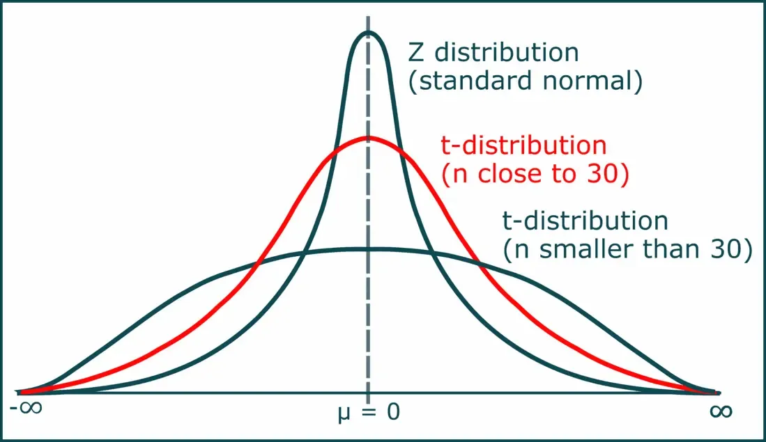
This figure shows how t-distribution curves change with degrees of freedom, illustrating how the sampling distribution narrows and approaches normality as df increases. Source.
Unlike the one-sample case, however, the degrees of freedom for the two-sample t-test do not follow a simple formula. The syllabus specifies that technology is used to estimate them, and these degrees of freedom lie between the smaller of (n1 − 1) and (n2 − 1) and the combined total (n1 + n2 − 2). This range reflects how uncertainty in estimating two variances affects the shape of the sampling distribution.
Interpreting the Magnitude of the Test Statistic
A larger magnitude of the t-value indicates stronger evidence against the null hypothesis.
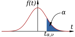
This diagram illustrates how a t-statistic is located on a t-distribution curve and how tail areas correspond to probabilities used to evaluate evidence against a null hypothesis. Source.
This occurs when:
the observed difference in sample means is large
the hypothesized difference is far from what the data suggest
the standard error is small due to low variability or large sample sizes
Because the t-statistic standardizes the observed difference, it allows meaningful comparisons across studies with different sample sizes or scales.
When to Use the Two-Sample t-Statistic
The test statistic described in this subsubtopic applies specifically when the following conditions are met:
Two samples are independent.
Each population is normally modeled, or sample sizes are sufficiently large for the sampling distribution to be approximately normal.
The population standard deviations are unknown, so the test must rely on sample statistics.
Key Considerations in Computation
The structure of the t-statistic emphasizes that statistical inference depends on both the size of the observed effect and the reliability of that estimate. Important points include:
A difference close to the hypothesized value results in a small t-statistic.
A difference far from the hypothesized value results in a large magnitude t-statistic.
Larger sample sizes decrease the standard error, making it easier to detect meaningful differences.
Unequal sample variances naturally influence the denominator, altering the strength of the evidence.
Students should recognize that the test statistic is the bridge between sample evidence and the inferential conclusion. It quantifies how incompatible the data are with the null hypothesis by measuring the standardized distance between what is observed and what is expected under the null model.
FAQ
When sample variances differ greatly, the standard error becomes dominated by the group with the larger variance. This increases the denominator of the test statistic, leading to a smaller magnitude t-value.
The test remains valid, but the evidence against the null hypothesis may weaken because the estimate of variability becomes larger.
Although most comparisons test whether the population means are equal, some research questions specify a particular expected difference. In these cases, the numerator subtracts this hypothesised difference rather than zero.
This allows the t-test to evaluate whether the observed difference departs meaningfully from a non-zero benchmark rather than simply testing equality.
The two-sample situation estimates two independent variances, each with its own uncertainty. Combining these uncertainties produces a more complex distribution shape.
For precision, statistical software uses the Welch–Satterthwaite approximation, producing a degrees-of-freedom value that adapts to sample sizes and variances.
Outliers inflate the sample standard deviation, which raises the standard error and reduces the magnitude of the t-value. This can mask genuine differences between population means.
Before computing the test statistic, it is good practice to check for unusual values and consider whether they reflect true population behaviour or measurement error.
Yes, the sign indicates the direction of the difference between sample means. A positive t-value suggests that sample 1 has a larger mean; a negative value suggests the opposite.
The magnitude determines strength of evidence, while the sign determines direction relative to the hypothesis being tested.
Practice Questions
Question 1 (1–3 marks)
A researcher collects two independent random samples to compare the mean reaction times of Group A and Group B. The sample statistics are:
Group A: x̄1 = 242 ms, s1 = 35 ms, n1 = 40
Group B: x̄2 = 259 ms, s2 = 42 ms, n2 = 38
The null hypothesis states that the population means are equal.
Calculate the test statistic for comparing the two means.
(Do not interpret the result.)
Question 1
• Correct substitution into the formula for the two-sample t-statistic:
t = (x̄1 − x̄2) / sqrt(s1²/n1 + s2²/n2). (1 mark)
• Correct calculation of the standard error. (1 mark)
• Correct final numerical value of the test statistic (allow minor rounding differences). (1 mark)
Question 2 (4–6 marks)
A nutritionist investigates whether two different training programmes lead to different mean weight gains. Two independent random samples are taken. The sample statistics are:
Programme 1: mean = 4.8 kg, standard deviation = 1.6 kg, n = 25
Programme 2: mean = 3.9 kg, standard deviation = 1.3 kg, n = 22
The nutritionist wishes to test the hypothesis that the two population means differ.
a) State the null and alternative hypotheses.
b) Calculate the test statistic for the difference in sample means.
c) Comment on whether the observed difference in sample means provides strong evidence against the null hypothesis, based solely on the magnitude of the test statistic (no p-value required).
Question 2
a)
• Null hypothesis stated correctly: H0: mean1 − mean2 = 0 or mean1 = mean2. (1 mark)
• Alternative hypothesis stated correctly: Ha: mean1 − mean2 ≠ 0. (1 mark)
b)
• Correct substitution into the two-sample t-statistic formula. (1 mark)
• Correct calculation of the standard error. (1 mark)
• Correct final numerical computation of the test statistic (allow minor rounding). (1 mark)
c)
• A clear statement that a larger magnitude t-value suggests stronger evidence against the null hypothesis, OR a correct qualitative assessment based on the computed value. (1 mark)
