
AQA Specification focus:
‘A supply curve shows the relationship between price and quantity supplied; higher prices imply higher profits and provide the incentive to expand production; the causes of shifts in the supply curve; under perfect competition, the supply curve is the marginal cost curve.’
The supply curve demonstrates how firms respond to different price levels, showing the relationship between price and quantity supplied, and explaining incentives and shifts under competitive conditions.
The Supply Curve
The supply curve illustrates the relationship between the price of a good or service and the quantity producers are willing to supply. It is generally upward sloping, reflecting that higher prices encourage firms to produce more output.
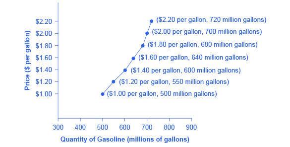
This diagram depicts a standard upward-sloping supply curve, reflecting the direct relationship between price and quantity supplied, where higher prices incentivize increased production. Source
Supply Curve: A graphical representation showing the relationship between the market price of a good and the quantity supplied by firms.
This positive relationship arises because higher prices typically allow firms to cover higher production costs and achieve greater profits.
Incentives and Profit Motive
A central reason the supply curve slopes upward is the profit incentive. When the price of a good increases, producers can expect:
Higher revenue from each unit sold.
Greater profit margins if costs remain stable.
Encouragement to reallocate resources towards production of that good.
The incentive to expand production underpins much of supply theory. Firms balance the potential revenue against costs when deciding how much to supply.
Shifts in the Supply Curve
A change in the market price leads to a movement along the supply curve, but other factors cause the whole supply curve to shift. These include:
Production costs: Increases in wages, raw material costs, or energy prices shift supply left (less supplied at each price).
Technological advances: More efficient production techniques shift supply right (more supplied at each price).
Taxes and subsidies: Indirect taxes increase costs and shift supply left; subsidies reduce costs and shift supply right.
Number of producers: An increase in firms supplying the market shifts supply right.
Expectations of future prices: Anticipation of higher future prices may reduce current supply.
External factors: Weather conditions or political instability can shift supply in agricultural or resource-based industries.
Shift in Supply: A change in the quantity supplied at every price level, caused by factors other than the good’s own price.
The Supply Curve and Marginal Cost
Under conditions of perfect competition, firms are price takers. This means that the supply curve of an individual firm corresponds to its marginal cost (MC) curve above the shutdown point.
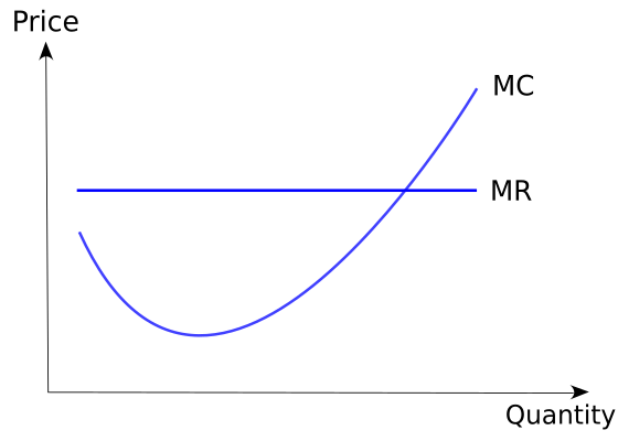
This diagram illustrates the marginal cost curve, which, in perfect competition, serves as the firm’s supply curve above the shutdown point, indicating the quantity supplied at each price level. Source
Marginal Cost: The additional cost incurred by producing one more unit of output.
The upward slope of the MC curve reflects the law of diminishing returns. As more units are produced, eventually additional inputs contribute less extra output, causing costs per unit to rise.
Perfect Competition and Supply
In a perfectly competitive market:
Firms face a perfectly elastic demand curve at the market price.
Profit maximisation occurs where marginal cost (MC) = marginal revenue (MR).
Since MR = Price under perfect competition, the supply decision depends on the MC curve.
The industry supply curve is the horizontal summation of all firms’ marginal cost curves.
This establishes a strong link between the microeconomic concept of costs and the market-level determination of supply.
Short-Run vs Long-Run Supply
The behaviour of supply differs between the short run and long run:
Short run: At least one factor of production is fixed. Supply is constrained, and shifts are often limited by capacity.
Long run: All factors are variable. Firms can adjust scale, enter or exit the market, leading to greater supply flexibility.
Shifts in supply are more pronounced in the long run, as firms can fully respond to incentives by expanding production or leaving unprofitable markets.
Key Influences on Supply Elasticity
The responsiveness of quantity supplied to price changes is known as price elasticity of supply (PES). Although calculation is covered elsewhere, it is important to note here that:
If supply is highly elastic, small price rises cause large increases in output.
If supply is inelastic, output responds little to price changes.
Factors influencing elasticity include:
Time period: Supply becomes more elastic in the long run.
Spare capacity: High unused capacity makes supply more elastic.
Ease of factor mobility: Flexible resources allow quick responses.
Perishability of goods: Perishable goods often have inelastic supply.
Linking Incentives and Market Outcomes
The supply curve demonstrates how incentives drive production decisions. For firms:
Rising prices increase willingness to supply.
Falling prices may lead to reduced output or market exit.
Shifts in costs or conditions change the whole curve, altering market outcomes.
Through these mechanisms, supply interacts with demand to determine market equilibrium — but always constrained by the underlying relationship between prices, costs, and incentives.
Practice Questions
Define what is meant by the term marginal cost. (2 marks)
1 mark for identifying it relates to the additional cost of producing one more unit of output.
1 mark for clarity that it is measured per unit (e.g. "the cost of producing an extra unit").
Explain why the supply curve of a firm in perfect competition corresponds to its marginal cost curve above the shutdown point. (6 marks)
Up to 2 marks for recognising that in perfect competition firms are price takers.
Up to 2 marks for explaining that firms maximise profit where price (marginal revenue) equals marginal cost.
Up to 1 mark for noting that the MC curve above average variable cost reflects the quantities a firm is willing to supply at different prices.
Up to 1 mark for linking explicitly to the idea that this makes the MC curve the firm's supply curve above the shutdown point.
FAQ
If firms expect future input costs (like wages or energy) to rise, they may increase current supply to avoid higher costs later.
Alternatively, if costs are expected to fall due to technological improvements, firms may delay production, shifting current supply left.
Expectations therefore influence whether supply today expands or contracts, even before actual costs change.
The shutdown point is where price just covers average variable cost.
If price falls below this point, the firm cannot cover variable costs, so it ceases production in the short run.
Above this point, the marginal cost curve shows the quantities firms are willing to supply at different prices.
Thus, the MC curve only represents supply above the shutdown level.
In the short run, at least one factor of production is fixed. As more variable inputs are added, additional output eventually increases at a decreasing rate.
This rising marginal cost results in an upward-sloping supply curve. Without diminishing returns, costs might not increase in the same way, and supply would look different.
Several policy measures affect supply conditions:
Indirect taxes (like VAT) raise production costs, shifting supply left.
Subsidies reduce costs, shifting supply right.
Regulations (such as safety or environmental standards) increase compliance costs, shifting supply left.
These policies directly alter firms’ willingness or ability to supply at each price.
In perfect competition, firms are price takers, so they can only adjust output to maximise profit where price equals marginal cost.
In imperfect competition, firms face downward-sloping demand curves. This means their output decisions are influenced by both price-setting behaviour and marginal cost.
As a result, only in perfect competition does the marginal cost curve act as the supply curve.
