
AQA Specification focus:
‘The difference between the short run and the long run; the difference between marginal, average and total returns; the law of diminishing returns; these relationships explain how inputs relate to output.’
Introduction
This section explores how firms convert inputs into outputs, examining differences between short run and long run, measures of returns, and the law of diminishing returns.
The Short Run and the Long Run
Short Run
In economics, the short run is defined as the period of time during which at least one factor of production is fixed. Typically, capital such as machinery or factory size is fixed, while labour and raw materials are variable.
Short Run: The time period in which at least one factor of production is fixed, and firms can only adjust variable inputs.
Firms in the short run are constrained by their existing capacity, which limits how much output can be increased.
Long Run
By contrast, the long run is when all factors of production are variable. Firms can adjust plant size, technology, and labour, enabling full flexibility in production decisions.
Long Run: The time period in which all factors of production are variable, allowing firms to change both scale and capacity.
The key difference is flexibility: in the short run, firms can only alter variable factors, but in the long run, they can expand or reduce overall scale.
Marginal, Average and Total Returns
Total Returns
Total returns refer to the total amount of output produced from a given quantity of inputs. It represents overall productivity generated by labour or other variable inputs.
Total Returns: The total amount of output produced by all units of a variable factor employed.
Average Returns
Average returns measure output per unit of a variable factor input, such as labour. It is found by dividing total output by the number of inputs used.
Average Returns (AR) = Total Output ÷ Units of Variable Input
AR = Output per worker (when labour is the input)
Average returns are useful for comparing efficiency across different levels of input.
Marginal Returns
Marginal returns indicate the additional output produced when one more unit of a variable factor is employed, holding all other factors constant.
Marginal Returns: The additional output generated by employing one more unit of a variable factor, with all other factors fixed.
Marginal Returns (MR) = Change in Total Output ÷ Change in Variable Input
The marginal return curve typically rises initially, reaches a peak, and eventually declines due to the law of diminishing returns.
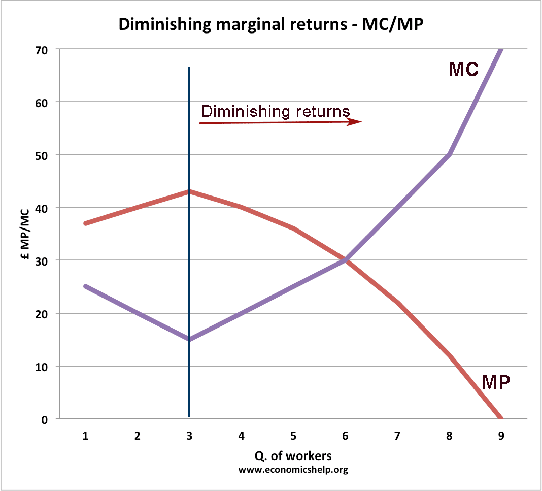
This graph shows the inverse relationship between marginal product (MP) and marginal cost (MC) as more labour is employed. MP initially rises, reducing MC, but eventually falls, causing MC to increase — illustrating the law of diminishing returns. Source
The Law of Diminishing Returns
Concept and Application
The law of diminishing returns states that if additional units of a variable factor (such as labour) are added to fixed factors (like capital or land), the marginal output from each extra unit will eventually decrease.
Law of Diminishing Returns: As more units of a variable factor are added to fixed factors, the additional output (marginal return) from each unit will eventually decline.
This principle only applies in the short run, since the presence of at least one fixed factor is essential for diminishing returns to occur.
Stages of Diminishing Returns
The process unfolds in identifiable phases:
Increasing returns: Initially, adding more workers may improve productivity as tasks are divided and efficiency improves.
Diminishing returns: Eventually, fixed capital becomes overused, so each new worker contributes less additional output.
Negative returns: If too many workers are employed, overcrowding reduces total output.
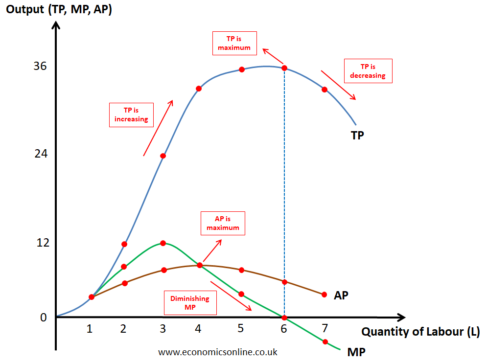
This diagram illustrates the relationship between total product (TP), marginal product (MP), and average product (AP). TP increases at first, then slows and falls, while MP and AP reflect the stages of increasing, diminishing, and negative returns. Source
Graphical Relationships between Returns
Total Returns (TR): Initially rises rapidly, then slows as diminishing returns set in, and can eventually fall if negative returns occur.
Average Returns (AR): Follows the total returns curve, rising at first and then falling as diminishing returns reduce output per worker.
Marginal Returns (MR): Always intersects the average returns curve at its maximum point, falling more quickly once diminishing returns set in.
These relationships are central to understanding how firms adjust input use in the short run.
Importance in Economic Analysis
Understanding the differences between short run and long run, and the concepts of total, average and marginal returns, is critical for:
Explaining why production efficiency changes as inputs vary.
Analysing cost behaviour, since returns influence average and marginal costs.
Demonstrating the constraints firms face in the short run due to fixed factors.
Showing how the law of diminishing returns underpins the upward slope of short-run cost curves in production theory.
Practice Questions
Define the law of diminishing returns and state in which time period it applies. (2 marks)
1 mark for a correct definition: As additional units of a variable factor are added to a fixed factor, the marginal output of each extra unit eventually decreases.
1 mark for correctly identifying the time period: Short run.
Using a diagram, explain the relationship between marginal product and average product in the short run. (6 marks)
1 mark for correctly drawing and labelling the marginal product (MP) and average product (AP) curves.
1 mark for showing that the MP curve rises initially, peaks, and then falls due to diminishing returns.
1 mark for showing that the AP curve follows a similar pattern but lags behind MP.
1 mark for correctly identifying that MP intersects AP at the maximum point of AP.
1 mark for explaining that when MP is above AP, AP rises, and when MP is below AP, AP falls.
1 mark for linking the behaviour of the curves to the law of diminishing returns.
FAQ
The law of diminishing returns requires at least one fixed factor of production. In the long run, all factors are variable, meaning firms can adjust plant size, technology, or labour to prevent overcrowding of resources.
Instead of diminishing returns, long-run analysis focuses on returns to scale, which considers how output changes when all inputs increase proportionally.
In agriculture, adding more fertiliser to a fixed plot of land initially boosts crop yield, but eventually each extra unit of fertiliser produces smaller gains.
In manufacturing, employing extra workers in a factory with limited machinery may first improve efficiency, but as more workers join, congestion lowers output per worker.
In the increasing returns phase: Total, average, and marginal returns all rise.
At the onset of diminishing returns: Marginal returns fall first, followed by average returns.
In negative returns: Marginal returns become negative, and total returns eventually decline.
When marginal product (MP) is higher than average product (AP), it pulls AP upwards.
Once MP falls below AP, it drags the average down. The exact point of intersection is where AP is maximised, reflecting the efficiency threshold of variable input use.
As marginal returns fall, more variable inputs are needed to produce each extra unit of output.
This leads to rising marginal cost (MC) and average cost (AC) curves in the short run.
The law of diminishing returns therefore directly underpins the upward slope of short-run cost curves used in production and cost analysis.
