
AQA Specification focus:
‘Returns to scale; the difference between increasing, constant and decreasing returns to scale; understand that these relationships have implications for costs of production.’
Introduction
Returns to scale analyse how output changes when all inputs are varied together. They explain efficiency in production and have direct consequences for long-run costs.
Understanding Returns to Scale
Definition of Returns to Scale
When studying production, economists examine how output responds to a proportional change in all factor inputs in the long run, when no factors are fixed.
Returns to Scale: The relationship between the proportional increase in factor inputs and the resulting change in output in the long run.
Returns to scale are crucial in understanding how firms expand and how costs behave when scaling up production.
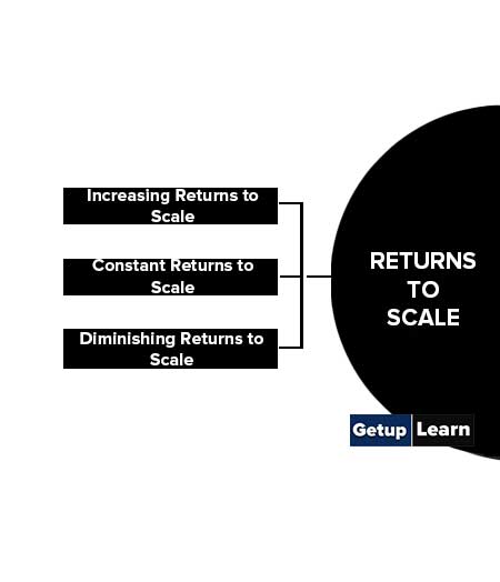
This diagram illustrates the three types of returns to scale: increasing, constant, and decreasing. It shows how output responds to proportional changes in all inputs, highlighting the corresponding effects on long-run average costs. Note that the diagram includes labels for iso-product curves and expansion paths, which are useful for understanding the graphical representation of returns to scale. Source
Types of Returns to Scale
Increasing Returns to Scale (IRS)
Occurs when output increases by a greater proportion than the increase in inputs.
Example: Doubling labour and capital causes output to more than double.
Implication: Firms experience falling long-run average costs, encouraging growth and efficiency.
Constant Returns to Scale (CRS)
Occurs when output increases in exact proportion to the increase in inputs.
Example: Doubling all inputs results in output that exactly doubles.
Implication: Long-run average costs remain unchanged.
Decreasing Returns to Scale (DRS)
Occurs when output increases by a smaller proportion than the increase in inputs.
Example: Doubling inputs leads to output rising by less than double.
Implication: Long-run average costs increase, discouraging further expansion.
Returns to Scale and Costs of Production
Connection to Long-Run Costs
In the long run, firms can adjust all factors of production. The cost implications are tied directly to the type of returns to scale:
Increasing returns to scale → Falling long-run average costs (LRAC).
Constant returns to scale → Stable LRAC.
Decreasing returns to scale → Rising LRAC.
This relationship explains the shape of the long-run cost curve and helps firms determine their efficient scale of operation.
Long-Run Average Cost Curve (LRAC)
The LRAC curve is influenced by returns to scale and reflects the cost per unit when all inputs are variable:
IRS produces the downward-sloping section of the LRAC.
CRS creates the flat portion where LRAC is constant.
DRS explains the upward-sloping section where LRAC increases.
The LRAC is often depicted as U-shaped, though modern theories suggest it can also appear L-shaped, reflecting extended periods of constant or falling costs.
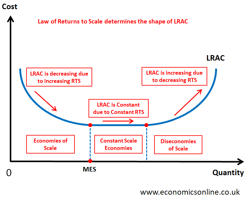
This diagram depicts the long-run average cost curve, illustrating the effects of increasing, constant, and decreasing returns to scale. The curve shows how average costs decrease, remain constant, or increase as output expands, reflecting the firm's scale of production. The diagram includes labels for economies of scale, constant returns to scale, and diseconomies of scale, providing a clear visual representation of these concepts. Source
Implications of Returns to Scale
Efficiency and Competitiveness
Firms achieving increasing returns to scale gain a cost advantage, enabling them to lower prices and improve competitiveness.
Industries with significant IRS (e.g., manufacturing, technology) tend to have fewer but larger firms.
Market Structure
Where IRS are strong, industries often become oligopolistic or monopolistic due to cost advantages from large-scale production.
CRS industries may remain fragmented, supporting many firms of varying sizes.
DRS discourages expansion beyond a certain size, influencing industry balance.
Barriers to Entry
High minimum efficient scale (MES) — the lowest output level at which LRAC is minimised — creates barriers to entry. New firms must enter at large scale to be competitive.
Returns to scale therefore influence market contestability and long-term industry dynamics.
Key Distinctions Between Short Run and Long Run
Short Run
Some factors are fixed, so firms face diminishing returns to a factor rather than returns to scale.
The law of diminishing returns explains cost patterns when only one input is increased.
Long Run
All inputs are variable, making returns to scale the governing concept.
Unlike diminishing returns, which occur due to input imbalance, returns to scale stem from proportional changes in all resources.
Factors Influencing Returns to Scale
Several factors explain why firms may experience different returns to scale:
Managerial Efficiency: Larger firms can specialise management tasks, improving decision-making.
Technical Factors: Larger machinery or advanced technology may only be feasible at higher output.
Financial Factors: Larger firms may access credit on better terms.
Coordination Challenges: As firms grow excessively, communication breakdowns and bureaucracy can cause diseconomies, leading to decreasing returns.
These elements help determine whether scaling up production is cost-effective.
Summary Points for Students
Returns to scale occur only in the long run.
Increasing returns reduce LRAC, constant returns maintain LRAC, and decreasing returns increase LRAC.
They directly shape the long-run average cost curve.
Implications include efficiency, competitiveness, barriers to entry, and industry structure.
Distinguish clearly between diminishing returns (short run) and returns to scale (long run).
Practice Questions
Define increasing returns to scale and explain briefly what happens to long-run average costs when a firm experiences this. (2 marks)
1 mark: Correct definition of increasing returns to scale (output increases by a greater proportion than inputs).
1 mark: Correct explanation that long-run average costs fall when increasing returns to scale occur.
Using an appropriate diagram, explain the relationship between returns to scale and the shape of the long-run average cost curve. (6 marks)
1 mark: Correctly identifies increasing returns to scale and links it to falling LRAC.
1 mark: Correctly identifies constant returns to scale and links it to flat LRAC.
1 mark: Correctly identifies decreasing returns to scale and links it to rising LRAC.
1 mark: Reference to the LRAC being U-shaped (or L-shaped under modern theory).
1 mark: Clear explanation of how changes in input-output proportions drive these cost changes.
1 mark: Clear and accurately labelled diagram showing LRAC curve with sections linked to returns to scale.
FAQ
Industries with high fixed costs and the ability to spread those costs over a large output often experience increasing returns to scale.
Examples include:
Car manufacturing, where expensive machinery is used more efficiently at higher output levels.
Technology and software, where development costs are large but replication is cheap.
Energy supply, where infrastructure investment benefits from larger-scale usage.
These industries typically see falling long-run average costs as they grow.
As firms grow larger, managing resources becomes more complex. Communication may slow down, decision-making layers multiply, and workers can feel less motivated.
This lack of coordination and rising bureaucracy increases inefficiency. Eventually, output rises by a smaller proportion than inputs, pushing long-run average costs upward.
Returns to scale describe the technical relationship between input and output when all inputs change proportionally.
Economies of scale focus on cost advantages, such as lower average costs due to bulk buying or specialisation.
In short:
Returns to scale = output changes.
Economies of scale = cost changes.
The two concepts are linked, but not identical.
Yes. A firm may initially experience increasing returns to scale as it grows, then constant returns once efficiency peaks, and eventually decreasing returns due to diseconomies.
This shift explains why the long-run average cost curve can be U-shaped. The exact point where transitions occur depends on technology, management, and the nature of production.
Technology is central to returns to scale because it affects how inputs combine to generate output.
Advanced machinery may enable higher productivity at larger scale.
Automation reduces reliance on labour, increasing the potential for increasing returns.
Outdated technology may limit efficiency, making decreasing returns more likely at lower levels of output.
Thus, investment in modern production methods can extend the range over which firms experience increasing returns.
