Instantaneous rate of change captures how a quantity evolves at a single moment, extending the idea of average rate of change through the powerful concept of limits central to calculus.

Understanding Change at an Instant

When studying changing quantities, students first encounter average rate of change, which measures how one variable varies with respect to another over a finite interval. However, many real-world situations—such as velocity at a specific time or chemical concentration at a precise moment—require understanding change at an instant, not over a span. This leads naturally to the idea of the instantaneous rate of change, a foundational concept in calculus.

As the time interval becomes smaller, the average rate describes increasingly localized behavior. The progression from a coarse measurement to an extremely precise one relies on the mathematical machinery of limits.

Connecting Average and Instantaneous Rates Using Limits

To understand instantaneous behavior, begin with the average rate of change of a function f between two points. As the horizontal distance between those points shrinks, the average rate reveals the dynamic change occurring at a single input value.

This expression becomes a bridge to instantaneous change when students examine what happens as $h$ becomes very small. The limit captures this idea rigorously by examining how the expression behaves as $h$ approaches zero. In doing so, the limit describes the rate of change at an exact moment, not over an interval.

Between definition and application, it is essential to see limits not as a computational tool but as a conceptual framework: they describe the behavior of a function as one variable approaches another value, even if the function never actually reaches that value.

Why Limits Are Essential for Instantaneous Change

The instantaneous rate of change cannot be computed directly by substituting $h = 0$ into the average rate formula, because this would lead to a denominator of zero. Instead, the limit evaluates the behavior near zero, allowing us to extract meaningful information about the function's behavior at a specific input.

Key reasons limits are necessary include:

• Avoiding undefined expressions by examining behavior rather than direct substitution.

• Capturing dynamic behavior, such as velocity at a single moment during motion.

• Generalizing change across many contexts, such as population growth or temperature variation.

Discussing limits in this context reinforces their role in transforming average measurements into precise, instantaneous ones. A limit formalizes the idea of “approaching” without requiring exact equality, allowing calculus to describe scenarios that algebra alone cannot express.

The Limit as Intervals Shrink

The central process in finding instantaneous rate of change is shrinking the interval between two points on a graph. As the second point moves closer to the first, the slope of the secant line between them approaches the slope of the tangent line at the point of interest.

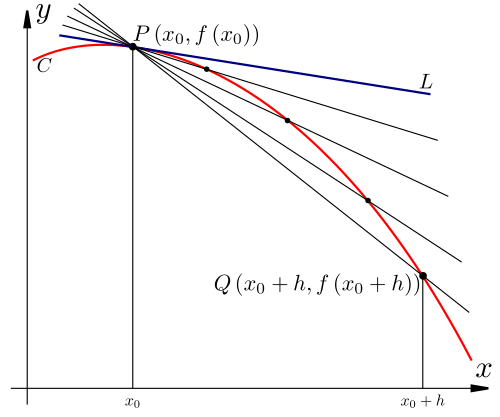
This diagram shows a curve with secant lines approaching the tangent line as the interval shrinks, illustrating how instantaneous rate of change arises from the limit of average rates. Source.

Although graphical interpretations are not computed here, this conceptual picture supports the analytic definition.

Important relationships in this shrinking-interval perspective include:

• The distance between the two $x$-values becomes extremely small.

• The numerator $f(x+h) - f(x)$ measures increasingly subtle change in output.

• The ratio of these quantities trends toward a stable value if the function behaves smoothly.

Because of this, limits model real-world dynamic processes such as instantaneous velocity in physics, marginal cost in economics, or concentration change in chemistry.

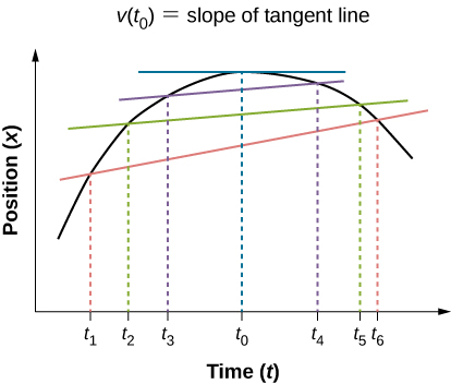
This graph shows average velocities as slopes of secant lines and instantaneous velocity as the slope of the tangent line, demonstrating how limits describe motion at a precise moment. Source.

Limits as a Unifying Framework for Dynamic Contexts

In many applied situations, change is continuous rather than abrupt. The limit-based definition of instantaneous rate of change allows students to describe:

• How quickly an object is moving at a specific moment.

• How a biological population is changing at a particular time.

• The rate at which a chemical reaction proceeds at a precise concentration.

These contexts highlight why calculus is essential for modeling natural and human-made systems.

Students should recognize that the same limit concept underpins all such interpretations, regardless of the specific phenomenon being analyzed.

The Importance of Approaching, Not Equaling

A crucial conceptual shift is realizing that the input does not need to equal the target value. The limit describes behavior near the value of interest, enabling analysis even when the function is undefined at that exact point. This framing helps students appreciate the flexibility and power of limits in capturing instantaneous behavior where algebraic tools fail.

Bullet points reinforcing this idea include:

• The function need not be defined at the point where the instantaneous rate is evaluated.

• What matters is predictable, stable behavior as inputs get arbitrarily close.

• Limits allow functions with holes, jumps, or other discontinuities to still exhibit meaningful trends nearby.

This viewpoint aligns with the AP requirement to use limits to model dynamic change and supports later work with derivatives, which formalize instantaneous rate of change.

Limits as the Foundation for Further Calculus Concepts

Instinctively, students may imagine instantaneous change as an intuitive notion; however, its mathematical definition depends entirely on limits. By grounding the concept in limit processes, they build a robust foundation for derivative rules, motion models, optimization, and differential equations. Understanding instantaneous rate of change through limits establishes a coherent pathway into the core ideas of calculus, linking numerical, graphical, and conceptual reasoning around dynamic change.