Average rate of change describes variation over intervals, but at a single instant the interval collapses, making division impossible and leading naturally to the limiting idea of instantaneous change.

Why Average Rates Fail at a Single Instant

Understanding Average Rate of Change

The average rate of change of a function over an interval compares how much a quantity changes relative to a change in the independent variable. It is conceptually tied to the idea of dividing a net change by the length of the interval.

Because this concept relies on comparing two distinct points, it inherently requires a nonzero horizontal distance between those points. When an interval shrinks to a single point, the computation no longer makes sense.

Average rates are widely used to describe motion, population change, profit variation, or temperature change, all of which depend on observing behavior over measurable stretches of time or space.

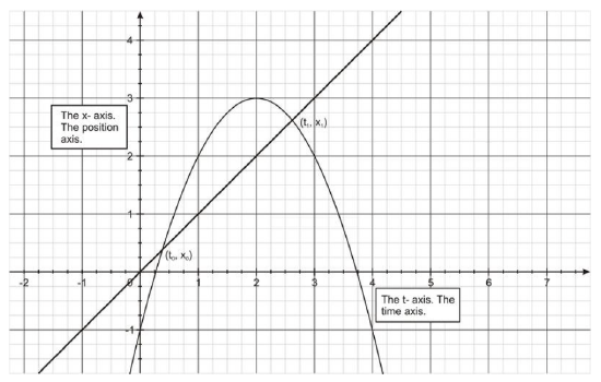
The graph shows a position–time curve with a secant line whose slope represents the average velocity over the interval. Labels identify the two points used to compute the average rate of change. The axes are marked to clarify the physical meaning of position and time. Source.

Why Average Rate of Change Cannot Be Computed at a Single Point

At a single instant, the change in the independent variable is zero, creating a division by zero situation. Since dividing by zero is undefined, no meaningful value can be assigned to the average rate at a single point. This aligns directly with the syllabus requirement that students recognize the failure of average rate of change at a single point.

The breakdown occurs because average rate of change is inherently a two-point measurement; collapsing to one point removes the comparison needed to compute change.

Key reasons the average rate fails at an instant include:

• It requires two distinct input values, but a single instant provides only one.

• The denominator $\Delta x$ becomes zero, making the expression $\frac{\Delta y}{\Delta x}$ undefined.

• No interval means no measurable “over time” or “over distance” context to interpret the change.

From Breakdown to Motivation for Limits

The failure of average rate of change at a single instant motivates the introduction of the limit. Instead of attempting to compute change at a point directly, calculus considers what the average rate of change approaches as intervals become extremely small.

As $\Delta x$ shrinks, the ratio describing average behavior begins to approximate instantaneous behavior.

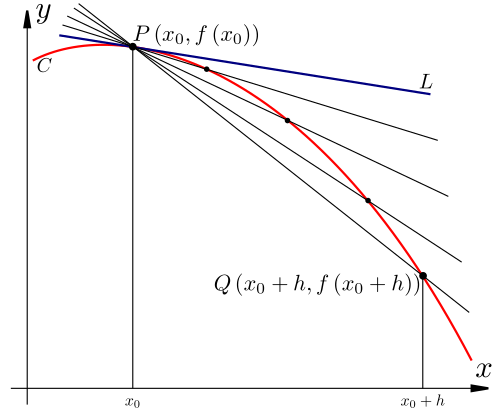
The diagram shows how the secant line between two nearby points on a curve approaches the tangent line as the interval shrinks. The shrinking horizontal distance hhh illustrates how average rates of change converge toward an instantaneous rate. This visual reinforces the limiting idea behind instantaneous change. Source.

The Structure Behind the Failure

The algebraic form of the average rate of change exposes why it cannot survive at an instant.

If $h = 0$, the denominator becomes zero, invalidating the expression. Thus, the formula itself demands that the interval length be nonzero. This algebraic restriction confirms the conceptual problem: change over “no interval” has no definable meaning.

A single point cannot encode variation, since variation is inherently relational. The average rate’s breakdown therefore highlights the need for a new conceptual tool that can describe behavior at an instant without requiring division by zero.

The Role of Nearby Behavior

To address this limitation, calculus focuses on what happens near the point rather than at the point. By examining values of the average rate of change for small positive and negative intervals around the target point, we gain insight into how the function behaves in the immediate vicinity.

This approach shifts attention from static measurement to dynamic approximation. The idea is that while an exact instantaneous rate cannot be computed directly, it may be approached by studying increasingly small intervals.

Key observations:

• The smaller the interval, the more closely the average rate mimics instantaneous behavior.

• Approaching a single point from both sides reveals whether the behavior stabilizes to a single predictable value.

• If the limiting value exists, it provides a meaningful description of instantaneous change.

Why the Limit Concept Resolves the Problem

Limits allow us to evaluate expressions that cannot be computed through direct substitution. In the context of rates, limits transform the undefined expression at $h = 0$ into a process-based evaluation of how the expression behaves as $h$ approaches zero.

This resolves the average rate breakdown by reframing the question:

• Not “What is the rate at a point using two distinct values?”

• But “What value do the average rates approach as the interval collapses?”

Through this lens, instantaneous change becomes both conceptually meaningful and mathematically precise, preparing students for the formal definition of the derivative in later topics.

The syllabus emphasis on why average rates fail at a single instant is foundational: it highlights the limitations of pre-calculus ideas and illuminates why the limit concept is essential for studying continuous change.