Horizontal asymptotes describe a function’s long-term behavior as the input grows without bound. Understanding limits at infinity reveals how functions settle toward constant values that govern end behavior.

Understanding Horizontal Asymptotes

Horizontal asymptotes arise when the output of a function approaches a constant value as x → ∞ or x → −∞.

This perspective focuses on end behavior, the long-run trend of a graph rather than its behavior near specific points. Students must recognize that horizontal asymptotes describe approach, not permanent confinement; a function may cross or move away from an asymptote yet still exhibit asymptotic behavior at infinity.

When studying end behavior, the guiding principle is that limits at infinity translate directly into statements about horizontal asymptotes. If a function settles toward a single numerical value as x becomes arbitrarily large in the positive or negative direction, that value defines a horizontal asymptote. These ideas align with the AP emphasis on connecting limit notation with graphical interpretation, enabling students to understand asymptotes as descriptors of long-term stability.

Limits at Infinity and Asymptotic Behavior

A limit at infinity describes the value a function approaches as x increases or decreases without bound. This concept underlies every determination of a horizontal asymptote. When the limit equals a real number, the corresponding horizontal line indicates the end behavior of the curve. A graph interpreted through this lens becomes a tool for predicting how a model behaves far into the future or at extreme input values.

Between positive and negative infinity, a function may approach different constant values. Therefore, it is essential to consider each direction separately, consistent with the syllabus requirement to determine horizontal asymptotes using limits as x approaches positive or negative infinity.

A single sentence must appear here before any other definition or equation to maintain proper formatting.

A function may have no horizontal asymptotes, one horizontal asymptote, or two distinct horizontal asymptotes depending on the values of the relevant limits.

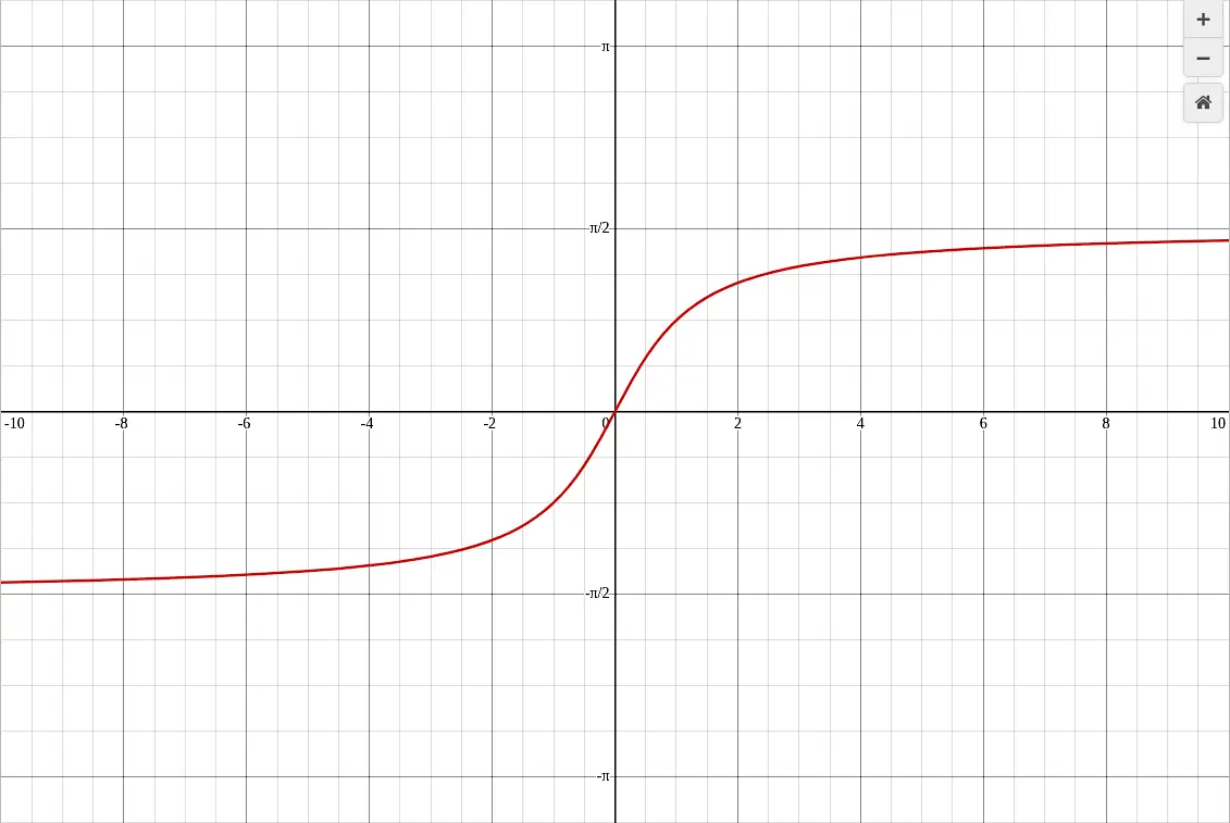
This graph of the arctangent function shows two horizontal asymptotes at $y=\frac{\pi}{2}$ and $y=-\frac{\pi}{2}$. As $x\to\infty$, the curve approaches the upper asymptote, and as $x\to -\infty$, it approaches the lower asymptote. The image includes inverse trigonometric detail that exceeds the syllabus slightly but remains aligned with AP Calculus AB expectations. Source.

These outcomes depend entirely on limit behavior, not on algebraic form alone.

A sentence is required between definition or equation blocks before continuing further.

These limit expressions emphasize that horizontal asymptotes are determined exclusively by end behavior, even when the function’s local features are more irregular.

Graphical Interpretation of Limits at Infinity

Interpreting limits visually helps students recognize horizontal asymptotes by observing whether the graph levels off as x moves toward large positive or negative values. The leveling tendency corresponds to the y-value that the curve nears, and this becomes the asymptotic value predicted by the limit notation.

Key Graphical Indicators

• The function’s output becomes increasingly stable as x grows large.
• Oscillations, if present, diminish toward a constant center value.
• The graph flattens and approaches a horizontal line.
• Distinct behaviors may appear on the left and right ends of the graph.

These interpretations reinforce the AP requirement to relate limit results to graphical asymptotic behavior and deepen conceptual understanding of how limits convey end behavior.

Analytical Strategies for Identifying Horizontal Asymptotes

Because AP Calculus AB expects students to determine horizontal asymptotes using limits at infinity, algebraic reasoning must support graphical observations. Through limit evaluation, students justify asymptotes rather than merely reading them from a graph.

Guiding Principles for Algebraic Determination

• Evaluate $\lim_{x\to\infty} f(x)$ and $\lim_{x\to -\infty} f(x)$ independently.
• Recognize that end behavior depends on dominant terms for expression types such as rational, exponential, logarithmic, or trigonometric functions.
• Use appropriate limit laws or algebraic manipulation when necessary to clarify long-term behavior.
• Interpret constant limit values as asymptotes and nonconstant or unbounded limits as indicating no horizontal asymptote for that direction.

These procedures integrate limit laws with conceptual understanding, consistent with AP expectations that students connect algebraic and graphical representations.

Conceptual Significance in Mathematical Modeling

Horizontal asymptotes often appear in models where quantities stabilize over time or after significant growth. The limit framework allows students to express stabilization precisely using asymptotic language. Whether modeling velocity, population growth, or cooling processes, the horizontal asymptote represents the equilibrium state that the model approaches as inputs become very large. This captures the essence of the syllabus emphasis on relating constant limit values to asymptotic behavior.

By mastering limits at infinity and understanding how they determine horizontal asymptotes, students develop a deeper and more versatile view of functions’ long-term behavior.