Limits at infinity describe how a function behaves as its input grows without bound, providing essential insight into long-term trends and the overall end behavior of functions.

Limits at Infinity

Understanding limits at infinity is central to analyzing how functions behave for extremely large positive or negative inputs. When we evaluate a limit as $x \to \infty$ or $x \to -\infty$, we are not looking for where the function ends—because it continues indefinitely—but rather the value the function’s output approaches. This behavior reveals patterns such as leveling off, unbounded growth, or decay.

When first discussing limits at infinity, it is important to connect the idea to the broader concept of a limit: investigating what value a function approaches, rather than what value it attains. Limits at infinity expand this notion to the “far ends” of the graph, allowing us to describe whether a function becomes arbitrarily large, settles near a constant value, or decreases without bound.

The Meaning of “End Behavior”

The end behavior of a function refers to how its output values behave as the input grows large in magnitude. End behavior focuses on trends rather than specific points and helps distinguish among different families of functions. It also provides a foundation for identifying horizontal asymptotes and comparing growth rates.

A function’s end behavior is typically represented graphically by how the curve extends toward the edges of the coordinate plane. Algebraically, it is described through limit notation, reflecting the value the function tends toward.

Limit Notation for End Behavior

Using limit notation emphasizes that the value approached is what matters, not whether it is ever reached. When we say $\lim_{x\to \infty} f(x)=L$, we are expressing that the function grows arbitrarily close to $L$ for sufficiently large $x$.

This notation reinforces that limits at infinity help determine whether the function stabilizes near a horizontal line or continues to grow.

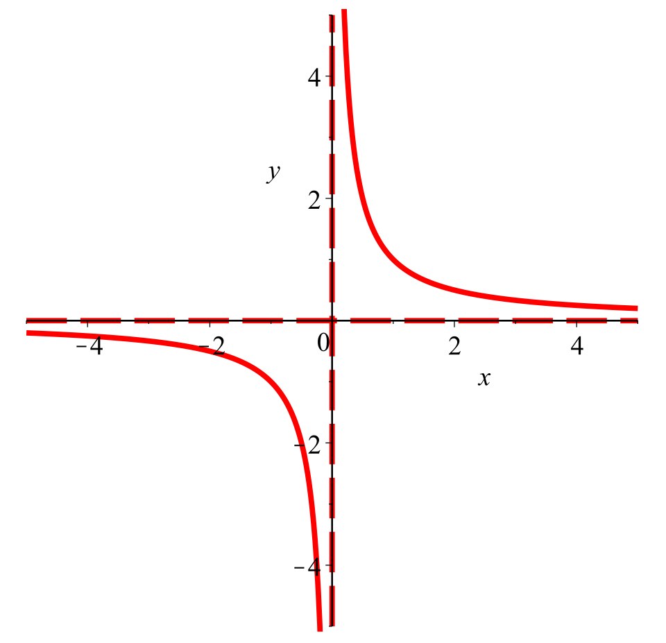
Graph of $f(x)=\frac{1}{x}$ with a horizontal asymptote at $y=0$ and a vertical asymptote at $x=0$. The arrows show that as $x\to\pm\infty$, the curve gets closer to the line $y=0$, illustrating a limit at infinity. The vertical asymptote indicates local unbounded behavior that extends slightly beyond this subsubtopic. Source.

Recognizing Different End Behaviors

While functions may display complex behavior near the origin or at particular points, their end behavior is often simpler and governed by dominant terms in their algebraic expressions. Common patterns include:

• Approaching a constant value, often indicating a horizontal asymptote.

• Increasing without bound as the input becomes large.

• Decreasing without bound as the input becomes large in magnitude.

• Oscillating while still approaching a limiting value.

These patterns provide a broad understanding of the categories into which many functions fall.

End Behavior of Common Function Families

Different types of functions exhibit predictably different behaviors at infinity. For AP Calculus AB, recognizing these patterns strengthens intuition and supports more advanced limit techniques.

Polynomial Functions

Polynomials exhibit end behavior driven by the term with the highest exponent. Lower-degree terms become negligible for large values of $|x|$, creating a clear pattern of growth or decay based on the leading coefficient and degree.

Because this dominant term controls behavior at infinity, polynomials do not level off; they grow without bound or fall without bound depending on sign and degree.

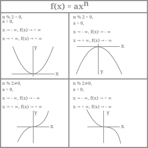
Four-panel diagram showing the end behavior of $f(x)=a x^n$ for even and odd degrees with positive and negative leading coefficients. Each panel illustrates how the graph behaves as $x\to\pm\infty$, contrasting “both ends up,” “both ends down,” and opposite-tail patterns. The labels refer specifically to monomials, a slightly narrower case that still directly represents polynomial end behavior. Source.

Rational Functions

Rational functions show more variety in end behavior, as the degrees of the numerator and denominator determine whether the function tends to zero, approaches a constant ratio, or grows without bound. When the denominator’s degree exceeds the numerator’s, outputs shrink toward zero, revealing a horizontal asymptote at $y=0$. When degrees match, the ratio of leading coefficients determines the value approached.

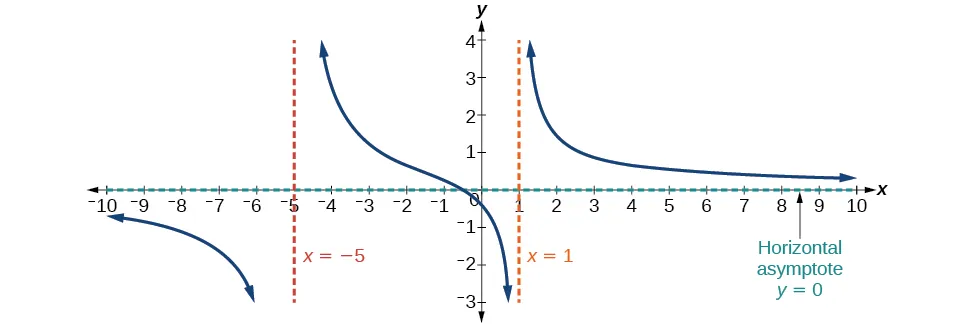
Graph of a rational function with vertical asymptotes at $x=-5$ and $x=1$ and a horizontal asymptote at $y=0$. The outer tails show the function approaching $0$ as $x\to\pm\infty$, demonstrating end behavior dominated by a higher-degree denominator. The vertical asymptotes provide additional context about local behavior not essential to the subsubtopic. Source.

Between these scenarios, rational functions illustrate how limits at infinity reveal nuanced asymptotic behavior not easily observed through local analysis.

Exponential and Logarithmic Functions

Exponential functions of the form $a^x$ with a>1 grow extremely rapidly as $x \to \infty$ and decay toward zero as $x \to -\infty$. Their consistent pattern makes them useful for modeling many real-world processes where growth accelerates over time.

Logarithmic functions, by contrast, grow without bound but do so extremely slowly. Even as $x$ becomes large, the output increases only incrementally, creating distinctive end behavior that contrasts sharply with exponential growth.

Using Limits at Infinity to Describe End Behavior

Limits at infinity provide precise language to describe long-term behavior, enabling statements such as:

• The function approaches a constant value.

• The function increases or decreases without bound.

• The function tends toward zero.

This approach allows for structured analysis of curves, supporting the interpretation of graphs, informing algebraic techniques, and connecting to broader concepts such as asymptotes and growth rates.