
AP Syllabus focus:
‘Explain how issues of scale or missing detail in a graph can hide important behavior, so estimated limits from a graph may not reflect the true behavior of the function.’
A graph’s appearance can misleadingly suggest limit behavior when scale choices or omitted details distort how closely the function approaches a value near a specific point.
Understanding How Graph Scale Affects Limit Estimation
Graphical limit estimation relies on observing the y-values a function appears to approach as x nears a chosen point. However, graphical representations are simplified visual models, and the way axes are scaled can greatly influence whether important features are visible. Because limits concern behavior arbitrarily close to a point, even small distortions in scale may cause students to infer incorrect limit values.
Vertical and Horizontal Scale Distortions
When a graph is stretched or compressed, essential features can become hidden.
Vertical compression can flatten the function’s apparent behavior, making it seem as though the function approaches a constant value even when subtle but important variation remains near the point of interest.
Vertical exaggeration can make bounded oscillations or minor deviations look like large fluctuations, suggesting nonexistence of a limit even when one exists.
Horizontal compression reduces the visible neighborhood around a point, causing sharp changes or discontinuities to appear instantaneous rather than gradual.
Horizontal stretching can obscure the rate at which function values approach a limit, making convergent behavior appear slower or nonexistent.
Because limits depend on behavior extremely close to a point, inadequate scaling may cause these fine details to disappear entirely.
Missing Detail and Graph Resolution Problems
A graph may fail to show behavior occurring in a very small interval, even if that behavior controls the true limit.
Hidden Oscillations or Rapid Changes
Important nuances such as oscillations, sharp turns, or narrow spikes can vanish when the plotted resolution is too coarse.
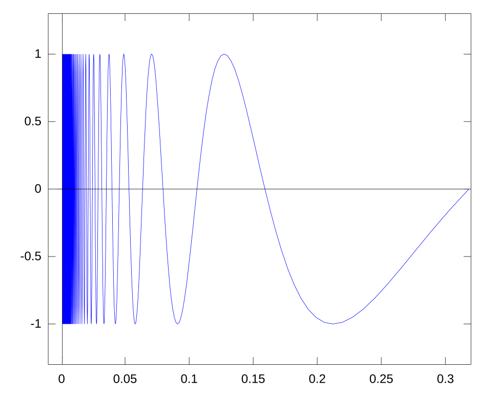
Graph of y=sin(1/x)y=\sin(1/x)y=sin(1/x) illustrating rapidly increasing oscillations near x=0x=0x=0. The oscillations remain bounded but become dense, demonstrating how limited graphical resolution can hide true limiting behavior. Source.
The plotting tool may skip over small intervals near the point of interest.
Sudden growth or rapid oscillation may exceed the graph’s sample density, causing the displayed curve to appear smooth.
Piecewise definitions or discontinuities may occur in intervals too small to display accurately with standard graphing resolution.
When such features are hidden, the estimated limit from the graph may not reflect the actual limiting behavior.
Misinterpretation of Apparent Function Values
Students sometimes assume that the drawn point or curve corresponds exactly to the function’s true behavior. Graphs, however, are approximations.
Open and Closed Points May Be Misleading
Graphing software or hand sketches may not accurately display whether a point is filled or unfilled.
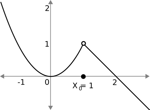
Diagram of a removable discontinuity showing a hole and a separate filled point at the same input value. This illustrates how drawn points may not accurately reflect either the function’s defined value or its limiting behavior. Source.
Open Point: A plotted circle indicating a value the function does not take at that -value.
A single drawn point does not guarantee correct representation of the function’s defined value. Even when open or closed points are depicted, they may be misaligned due to drawing imprecision. One cannot rely solely on the graphical mark to determine the function value at the point or the behavior arbitrarily close to it.
A graph may also include visual artifacts such as overlapping curves or thick plot lines that obscure the true value the function approaches.
How Scale Choice Can Hide Discontinuities
Discontinuities often appear only in a very narrow region. Poorly chosen scales can make a discontinuity look like a smooth connection.
Jump Discontinuities Obscured by Large Scale
A jump discontinuity occurs when left-hand and right-hand limits differ.
Jump Discontinuity: A discontinuity in which the left-hand limit and right-hand limit at a point exist but are unequal.
If the graph compresses the vertical axis too much, the jump may appear negligible or flattened into a seemingly continuous segment. Conversely, if the horizontal axis is too coarse, the jump may appear to occur at a slightly different location or may not be visible at all. Either situation can lead to an incorrect estimate of the limit.
A graph may also show overlapping lines at different scales, making it unclear which branch represents the actual behavior near the point of interest.
When Apparent Limit Behavior Does Not Match True Limit Behavior
Because limits focus on values approached, not necessarily attained, the visual depiction must reflect extremely small neighborhoods. Missing details can lead to misinterpretations such as:
Inferring that a function approaches a single value when it actually oscillates or diverges.
Believing a limit does not exist when hidden fine-scale behavior reveals convergence.
Misreading vertical behavior due to ambiguous scaling around steep slopes or vertical asymptotes.
Concluding a false horizontal alignment due to resolution that rounds or smooths numerical output.
Even small deviations in the displayed curve can mislead if they arise from plotting approximations rather than true function values.
Strategies for Avoiding Graph-Based Errors
To minimize the risk of misinterpreting limit behavior, students should analyze graphs carefully and critically.
Techniques for Improving Interpretation
Examine the graph at multiple scales to reveal hidden features.
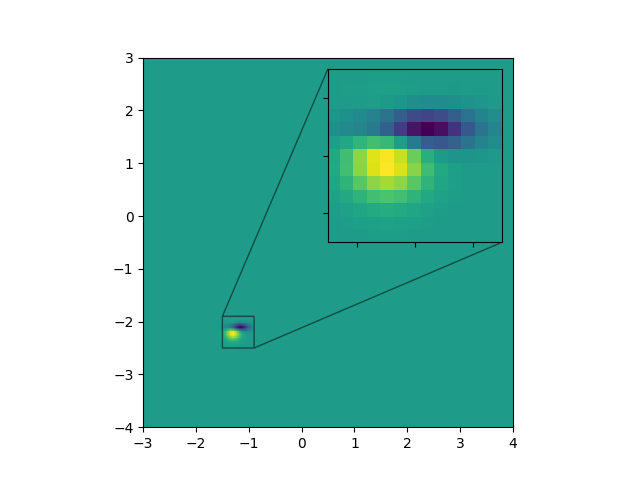
Main plot with an inset that magnifies a selected region, demonstrating how zooming reveals fine-scale structure invisible at the original scale. This reinforces why multiple scales are essential when estimating limits from graphs. Source.
Zoom in both vertically and horizontally to verify local behavior around the point of interest.
Compare the graph with numerical values or analytic expressions when available to confirm whether the observed behavior is genuine.
Check for plotting artifacts such as jagged edges, straight-line segments in nonlinear regions, or abrupt breaks caused by insufficient resolution.
Look for evidence of oscillation, divergence, or discontinuity that might not be apparent at the original scale.
These approaches help ensure that the limit estimation from a graph more closely reflects the true mathematical behavior.
Practice Questions
Question 1 (1–3 marks)
The graph of a function f is shown on a poorly scaled plot. Near x = 2, the graph appears to approach a single y-value. However, a more detailed graph reveals rapid oscillations of f in a very small interval around x = 2.
(a) State why the initial estimate of the limit as x approaches 2 may be unreliable.
(b) Explain how changing the graph’s scale could alter the interpretation of the limit.
Question 1
(a)
• 1 mark for stating that poor scaling or insufficient resolution can hide important behaviour such as oscillations or discontinuities.
• 1 mark for explaining that the limit estimate is unreliable because the true behaviour near x = 2 is not visible on the coarse graph.
(b)
• 1 mark for describing that adjusting vertical or horizontal scale (e.g., zooming in) may reveal hidden behaviour, changing the interpretation of the limit.
Question 2 (4–6 marks)
A student examines a graph of a function g and claims that the limit of g(x) as x approaches 0 exists and equals 3. The graph is drawn with coarse resolution and shows a curve that appears smooth near x = 0. A higher resolution graph suggests the following behaviours:
• g oscillates between 2.5 and 3.5 within 0.01 units of x = 0
• A removable discontinuity at x = 0 is not clearly marked on the lower resolution graph
• Zooming in horizontally reveals rapid changes in y-values that were not visible before
(a) Explain how missing detail in the coarse graph could lead the student to conclude incorrectly that a limit exists.
(b) Discuss how each of the three bullet points affects the interpretation of the limit.
(c) State, with justification, whether the limit of g(x) as x approaches 0 exists.
Question 2
(a)
• 1 mark for referring to low resolution masking oscillations or rapid changes.
• 1 mark for stating that hidden detail can make the graph appear to approach a single value when it does not.
(b)
• 1 mark for explaining that oscillations between 2.5 and 3.5 show the function does not stabilise near x = 0.
• 1 mark for explaining that a removable discontinuity, not visible on the coarse graph, affects whether the limit can be correctly identified.
• 1 mark for explaining that horizontal zoom reveals rapid variation, contradicting the apparent smoothness of the coarse graph.
(c)
• 1 mark for concluding that the limit does not exist because oscillations prevent the function from approaching a single value.
FAQ
Check whether the axes cover an unusually large range compared with the behaviour you are examining. Excessive stretching or compression often flattens oscillations or hides rapid changes.
Look for visual clues such as unusually straight segments in a curve that should not be linear, abrupt changes that seem too sharp, or a lack of visible detail near key x-values.
Commonly hidden features include:
• Small-scale oscillations
• Very narrow spikes or dips
• Rapid rate changes occurring in extremely small intervals
These behaviours may not be sampled correctly by plotting software, leading to a smoothed or oversimplified curve.
Graphing calculators often plot points at fixed intervals. If the discontinuity occurs between sampled points, the calculator may connect them with straight lines, disguising the break.
Limited pixel resolution can also position open or closed circles inaccurately, leading to incorrect interpretations of limit behaviour.
Be cautious when investigating limits near:
• Points where the formula involves division by very small numbers
• Expressions containing rapidly changing trigonometric or reciprocal terms
• Piecewise boundaries where behaviour may change abruptly
Smoothness on a graph does not guarantee smoothness in the underlying function.
Zooming helps, but it may still miss fine detail if the plotting algorithm does not increase sample density as you zoom.
In such cases, switching to numerical tables or using an algebraic approach often provides more reliable insight into the true limiting behaviour.
